Numpy: Arrays and Matrices

NumPy is an extension to the Python programming language, adding support for large, multi-dimensional (numerical) arrays and matrices, along with a large library of high-level mathematical functions to operate on these arrays.

Numpy functions are executed by compiled in C or Fortran libraries, providing the performance of compiled languages.

Sources: Kevin Markham

Computation time:

import numpy as np
import time

start_time = time.time()
l = [v for v in range(10 ** 8)]
s = 0
for v in l: s += v
print("Python code, time ellapsed: %.2fs" % (time.time() - start_time))

start_time = time.time()
arr = np.arange(10 ** 8)
arr.sum()
print("Numpy code, time ellapsed: %.2fs" % (time.time() - start_time))

Python code, time ellapsed: 6.13s
Numpy code, time ellapsed: 0.23s

Create arrays

Create ndarrays from lists. note: every element must be the same type (will be converted if possible)

data1 = [1, 2, 3, 4, 5]             # list
arr = np.array(data1)              # 1d array
data = [range(1, 5), range(5, 9)]  # list of lists
arr = np.array(data)              # 2d array
print(arr)
arr.tolist()                       # convert array back to list

[[1 2 3 4]
 [5 6 7 8]]

[[1, 2, 3, 4], [5, 6, 7, 8]]

Create special arrays

np.zeros(10)       # [0, 0, ..., 0]
np.zeros((3, 6))   # 3 x 6 array of zeros
np.ones(10)
np.linspace(0, 1, 5)            # 0 to 1 (inclusive) with 5 points
np.logspace(0, 3, 4)            # 10^0 to 10^3 (inclusive) with 4 points
np.arange(10)                   # [0, 1 ..., 9]

array([0, 1, 2, 3, 4, 5, 6, 7, 8, 9])

Examining arrays

print("Shape of the array: ",
      arr.shape)

print("Type of the array: ",
      arr.dtype)

print("Number of items in the array: ",
      arr.size)

print("Memory size of one array item in bytes: ",
      arr.itemsize)

# memory size of numpy array in bytes
print("Memory size of numpy array in bytes: %i, and in bits: %i" %
      (arr.size * arr.itemsize, arr.size * arr.itemsize * 8 ))

Shape of the array:  (2, 4)
Type of the array:  int64
Number of items in the array:  8
Memory size of one array item in bytes:  8
Memory size of numpy array in bytes: 64, and in bits: 512

Selection

arr[1, 2] # Get third item of the second line

np.int64(7)

Slicing

Syntax: start:stop:step with start (default 0) stop (default last) step (default 1)

• : is equivalent to 0:last:1; ie, take all elements, from 0 to the end with step = 1.

• :k is equivalent to 0:k:1; ie, take all elements, from 0 to k with step = 1.

• k: is equivalent to k:end:1; ie, take all elements, from k to the end with step = 1.

• ::-1 is equivalent to 0:end:-1; ie, take all elements, from k to the end in reverse order, with step = -1.

arr[0, :] # Get first line
arr[:, 2] # Get third column
arr[:, :2]     # columns strictly before index 2 (2 first columns)
arr[:, 2:]     # columns after index 2 included
arr2 = arr[:, 1:4]  # columns between index 1 (included) and 4 (excluded)
print(arr2)

# Slicing returns a view (not a copy)
# Modification

arr2[0, 0] = 33
print(arr2)
print(arr)

[[2 3 4]
 [6 7 8]]
[[33  3  4]
 [ 6  7  8]]
[[ 1 33  3  4]
 [ 5  6  7  8]]

Reverse order of row 0

print(arr[0, ::-1])

[ 4  3 33  1]

Fancy indexing: Integer or boolean array indexing

Fancy indexing returns a copy not a view.

Integer array indexing

arr2 = arr[:, [1, 2, 3]]  # return a copy
print(arr2)
arr2[0, 0] = 44
print(arr2)
print(arr)

[[33  3  4]
 [ 6  7  8]]
[[44  3  4]
 [ 6  7  8]]
[[ 1 33  3  4]
 [ 5  6  7  8]]

Boolean arrays indexing

arr2 = arr[arr > 5]  # return a copy

print(arr2)
arr2[0] = 44
print(arr2)
print(arr)

[33  6  7  8]
[44  6  7  8]
[[ 1 33  3  4]
 [ 5  6  7  8]]

However, In the context of lvalue indexing (left hand side value of an assignment) Fancy authorizes the modification of the original array

arr[arr > 5] = 0
print(arr)

[[1 0 3 4]
 [5 0 0 0]]

Array indexing return copy or view?

General rules:

• Slicing always returns a view.

• Fancy indexing (boolean mask, integers) returns copy

• lvalue indexing i.e. the indices are placed in the left hand side value of an assignment, provides a view.

Array manipulation

Reshaping

arr = np.arange(10, dtype=float).reshape((2, 5))
print(arr.shape)
print(arr.reshape(5, 2))

(2, 5)
[[0. 1.]
 [2. 3.]
 [4. 5.]
 [6. 7.]
 [8. 9.]]

Add an axis

a = np.array([0, 1])
print(a)
a_col = a[:, np.newaxis]
print(a_col)
#or
a_col = a[:, None]

[0 1]
[[0]
 [1]]

Transpose

print(a_col.T)

[[0 1]]

Flatten: always returns a flat copy of the original array

arr_flt = arr.flatten()
arr_flt[0] = 33
print(arr_flt)
print(arr)

[33.  1.  2.  3.  4.  5.  6.  7.  8.  9.]
[[0. 1. 2. 3. 4.]
 [5. 6. 7. 8. 9.]]

Ravel: returns a view of the original array whenever possible.

arr_flt = arr.ravel()
arr_flt[0] = 33
print(arr_flt)
print(arr)

[33.  1.  2.  3.  4.  5.  6.  7.  8.  9.]
[[33.  1.  2.  3.  4.]
 [ 5.  6.  7.  8.  9.]]

Stack arrays NumPy Joining Array

a = np.array([0, 1])
b = np.array([2, 3])

Horizontal stacking

np.hstack([a, b])

array([0, 1, 2, 3])

Vertical stacking

np.vstack([a, b])

array([[0, 1],
       [2, 3]])

Default Vertical

np.stack([a, b])

array([[0, 1],
       [2, 3]])

Advanced Numpy: reshaping/flattening and selection

Numpy internals: By default Numpy use C convention, ie, Row-major language: The matrix is stored by rows. In C, the last index changes most rapidly as one moves through the array as stored in memory.

For 2D arrays, sequential move in the memory will:

• iterate over rows (axis 0)

  • iterate over columns (axis 1)

For 3D arrays, sequential move in the memory will:

• iterate over plans (axis 0)

  • iterate over rows (axis 1)

    • iterate over columns (axis 2)

x = np.arange(2 * 3 * 4)
print(x)

[ 0  1  2  3  4  5  6  7  8  9 10 11 12 13 14 15 16 17 18 19 20 21 22 23]

Reshape into 3D (axis 0, axis 1, axis 2)

x = x.reshape(2, 3, 4)
print(x)

[[[ 0  1  2  3]
  [ 4  5  6  7]
  [ 8  9 10 11]]

 [[12 13 14 15]
  [16 17 18 19]
  [20 21 22 23]]]

Selection get first plan

print(x[0, :, :])

[[ 0  1  2  3]
 [ 4  5  6  7]
 [ 8  9 10 11]]

Selection get first rows

print(x[:, 0, :])

[[ 0  1  2  3]
 [12 13 14 15]]

Selection get first columns

print(x[:, :, 0])

[[ 0  4  8]
 [12 16 20]]

Ravel

print(x.ravel())

[ 0  1  2  3  4  5  6  7  8  9 10 11 12 13 14 15 16 17 18 19 20 21 22 23]

Vectorized operations

nums = np.arange(5)
nums * 10                           # multiply each element by 10
nums = np.sqrt(nums)                # square root of each element
np.ceil(nums)                       # also floor, rint (round to nearest int)
np.isnan(nums)                      # checks for NaN
nums + np.arange(5)                 # add element-wise
np.maximum(nums, np.array([1, -2, 3, -4, 5]))  # compare element-wise

# Compute Euclidean distance between 2 vectors
vec1 = np.random.randn(10)
vec2 = np.random.randn(10)
dist = np.sqrt(np.sum((vec1 - vec2) ** 2))

# math and stats
rnd = np.random.randn(4, 2) # random normals in 4x2 array
rnd.mean()
rnd.std()
rnd.argmin()                # index of minimum element
rnd.sum()
rnd.sum(axis=0)             # sum of columns
rnd.sum(axis=1)             # sum of rows

# methods for boolean arrays
(rnd > 0).sum()             # counts number of positive values
(rnd > 0).any()             # checks if any value is True
(rnd > 0).all()             # checks if all values are True

# random numbers
np.random.seed(12234)       # Set the seed
np.random.rand(2, 3)        # 2 x 3 matrix in [0, 1]
np.random.randn(10)         # random normals (mean 0, sd 1)
np.random.randint(0, 2, 10) # 10 randomly picked 0 or 1

array([0, 0, 0, 1, 1, 0, 1, 1, 1, 1])

Broadcasting

Sources: https://docs.scipy.org/doc/numpy-1.13.0/user/basics.broadcasting.html Implicit conversion to allow operations on arrays of different sizes. - The smaller array is stretched or “broadcasted” across the larger array so that they have compatible shapes. - Fast vectorized operation in C instead of Python. - No needless copies.

Rules

Starting with the trailing axis and working backward, Numpy compares arrays dimensions.

• If two dimensions are equal then continues

• If one of the operand has dimension 1 stretches it to match the largest one

• When one of the shapes runs out of dimensions (because it has less dimensions than the other shape), Numpy will use 1 in the comparison process until the other shape’s dimensions run out as well.

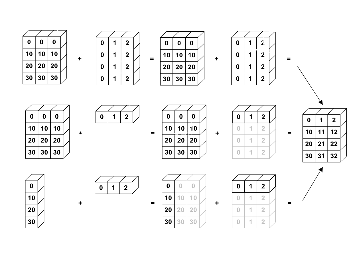
Source: http://www.scipy-lectures.org

a = np.array([[ 0,  0,  0],
              [10, 10, 10],
              [20, 20, 20],
              [30, 30, 30]])

b = np.array([0, 1, 2])

print(a + b)

[[ 0  1  2]
 [10 11 12]
 [20 21 22]
 [30 31 32]]

Center data column-wise

a - a.mean(axis=0)

array([[-15., -15., -15.],
       [ -5.,  -5.,  -5.],
       [  5.,   5.,   5.],
       [ 15.,  15.,  15.]])

Scale (center, normalise) data column-wise

(a - a.mean(axis=0)) / a.std(axis=0)

array([[-1.34164079, -1.34164079, -1.34164079],
       [-0.4472136 , -0.4472136 , -0.4472136 ],
       [ 0.4472136 ,  0.4472136 ,  0.4472136 ],
       [ 1.34164079,  1.34164079,  1.34164079]])

Examples

Shapes of operands A, B and result:

A      (2d array):  5 x 4
B      (1d array):      1
Result (2d array):  5 x 4

A      (2d array):  5 x 4
B      (1d array):      4
Result (2d array):  5 x 4

A      (3d array):  15 x 3 x 5
B      (3d array):  15 x 1 x 5
Result (3d array):  15 x 3 x 5

A      (3d array):  15 x 3 x 5
B      (2d array):       3 x 5
Result (3d array):  15 x 3 x 5

A      (3d array):  15 x 3 x 5
B      (2d array):       3 x 1
Result (3d array):  15 x 3 x 5

Exercises

Given the array:

X = np.random.randn(4, 2) # random normals in 4x2 array

• For each column find the row index of the minimum value.

• Write a function standardize(X) that return an array whose columns are centered and scaled (by std-dev).