Non-Linear Kernel Methods and Support Vector Machines (SVM)

import numpy as np
import pandas as pd
import seaborn as sns
import matplotlib.pyplot as plt

from sklearn.svm import SVC
from sklearn.preprocessing import StandardScaler

from sklearn import datasets
from sklearn import metrics
from sklearn.model_selection import train_test_split

# Plot
import matplotlib.pyplot as plt
import seaborn as sns

# Plot parameters
plt.style.use('seaborn-v0_8-whitegrid')
fig_w, fig_h = plt.rcParams.get('figure.figsize')
plt.rcParams['figure.figsize'] = (fig_w, fig_h * .5)

Kernel algorithms

Kernel Machine are based kernel methods require only a user-specified kernel function \(K(x_i, x_j)\), i.e., a similarity function over pairs of data points \((x_i, x_j)\) into kernel (dual) space on which learning algorithms operate linearly, i.e. every operation on points is a linear combination of \(K(x_i, x_j)\). Outline of the SVM algorithm:

1. Map points \(x\) into kernel space using a kernel function: \(x \rightarrow K(x, .)\). Learning algorithms operates linearly by dot product into high-kernel space: \(K(., x_i) \cdot K(., x_j)\).

   • Using the kernel trick (Mercer’s Theorem) replaces dot product in high dimensional space by a simpler operation such that \(K(., x_i) \cdot K(., x_j) = K(x_i, x_j)\).

   • Thus we only need to compute a similarity measure \(K(x_i, x_j)\) for each pairs of point and store in a \(N \times N\) Gram matrix of.

SVM

2. The learning process consist of estimating the \(\alpha_i\) of the decision function that maximizes the hinge loss (of \(f(x)\)) plus some penalty when applied on all training points.

3. Prediction of a new point \(x\) using the decision function.

\[f(x) = \text{sign} \left(\sum_i^N \alpha_i~y_i~K(x_i, x)\right).\]

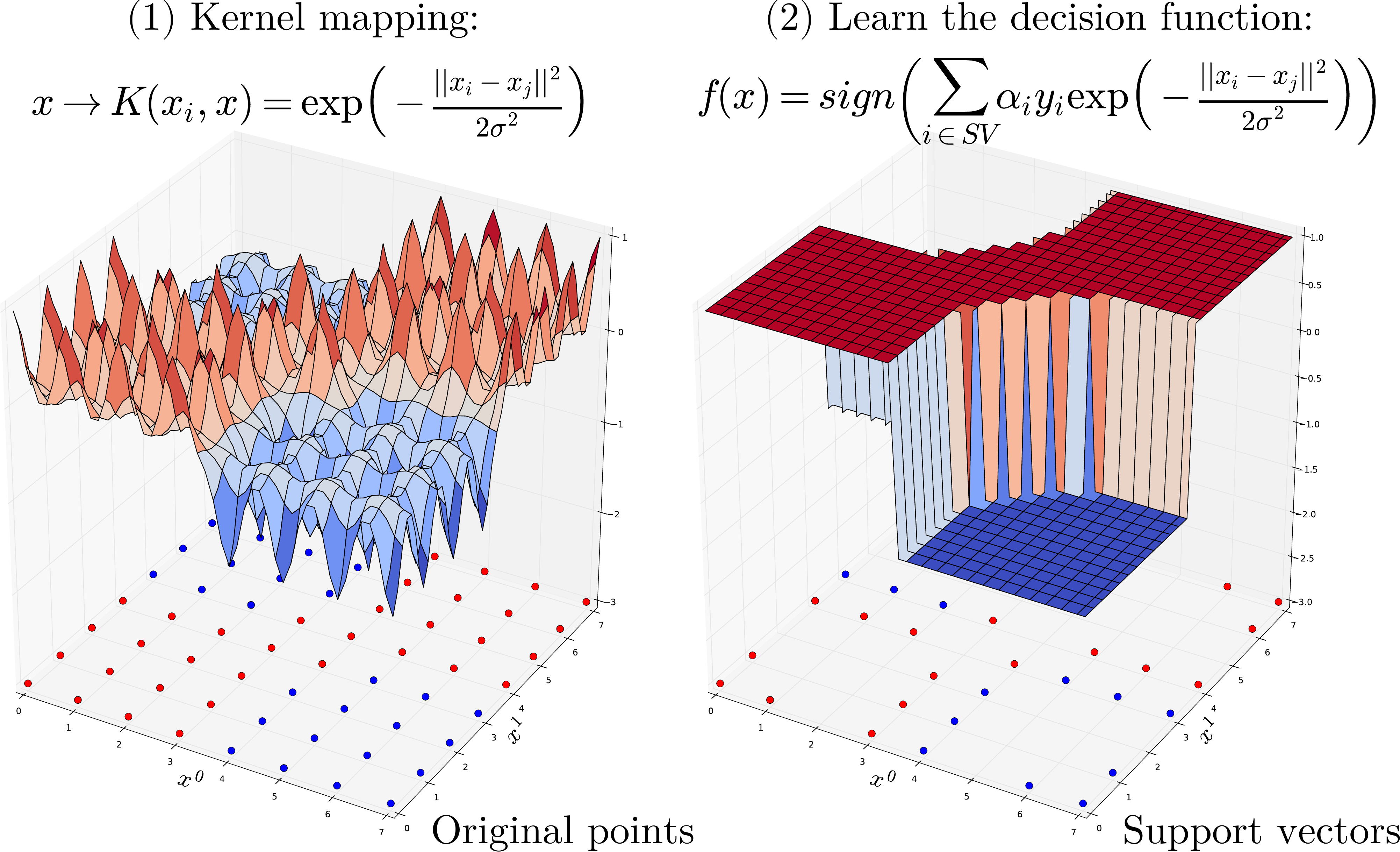
Kernel function

One of the most commonly used kernel is the Radial Basis Function (RBF) Kernel. For a pair of points \(x_i, x_j\) the RBF kernel is defined as:

Where \(\sigma\) (or \(\gamma\)) defines the kernel width parameter. Basically, we consider a Gaussian function centered on each training sample \(x_i\). it has a ready interpretation as a similarity measure as it decreases with squared Euclidean distance between the two feature vectors.

Non linear SVM also exists for regression problems.

Dataset

X, y = datasets.load_breast_cancer(return_X_y=True)
X_train, X_test, y_train, y_test = \
    train_test_split(X, y, test_size=0.5, stratify=y, random_state=42)

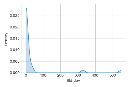
Preprocessing: unequal variance of input features, requires scaling for svm.

ax = sns.displot(x=X_train.std(axis=0), kind="kde", bw_adjust=.2, cut=0,
                 fill=True, height=3, aspect=1.5,)
_ = ax.set_xlabels("Std-dev").tight_layout()

scaler = StandardScaler()
X_train = scaler.fit_transform(X_train)
X_test = scaler.transform(X_test)

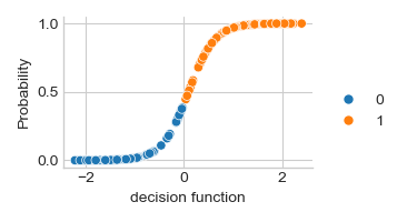
Scikit-learn SVC (Support Vector Classification) with probalility function applying a logistic of the decision_function

svm = SVC(kernel='rbf', probability=True).fit(X_train, y_train)
y_pred = svm.predict(X_test)
y_score = svm.decision_function(X_test)
y_prob = svm.predict_proba(X_test)[:, 1]

ax = sns.relplot(x=y_score, y=y_prob, hue=y_pred, height=2, aspect=1.5)
_ = ax.set_axis_labels("decision function", "Probability").tight_layout()

print("bAcc: %.2f, AUC: %.2f (AUC with proba: %.2f)" % (
      metrics.balanced_accuracy_score(y_true=y_test, y_pred=y_pred),
      metrics.roc_auc_score(y_true=y_test, y_score=y_score),
      metrics.roc_auc_score(y_true=y_test, y_score=y_prob)))

# Usefull internals: indices of support vectors within original X
np.all(X_train[svm.support_, :] == svm.support_vectors_)

bAcc: 0.96, AUC: 0.99 (AUC with proba: 0.99)

np.True_