Out-of-sample Validation for Model Selection and Evaluation

Source scikit-learn model selection and evaluation

from sklearn.base import is_classifier, clone
from joblib import Parallel, delayed
from sklearn.model_selection import StratifiedKFold
from sklearn.model_selection import cross_validate
from sklearn.model_selection import cross_val_score
from sklearn.model_selection import KFold
import numpy as np
import pandas as pd
import matplotlib.pyplot as plt
import seaborn as sns

from sklearn import datasets
import sklearn.linear_model as lm
from sklearn.model_selection import train_test_split, KFold, PredefinedSplit
from sklearn.model_selection import cross_val_score, GridSearchCV

import sklearn.metrics as metrics
X, y = datasets.make_regression(n_samples=100, n_features=100,
                                n_informative=10, random_state=42)

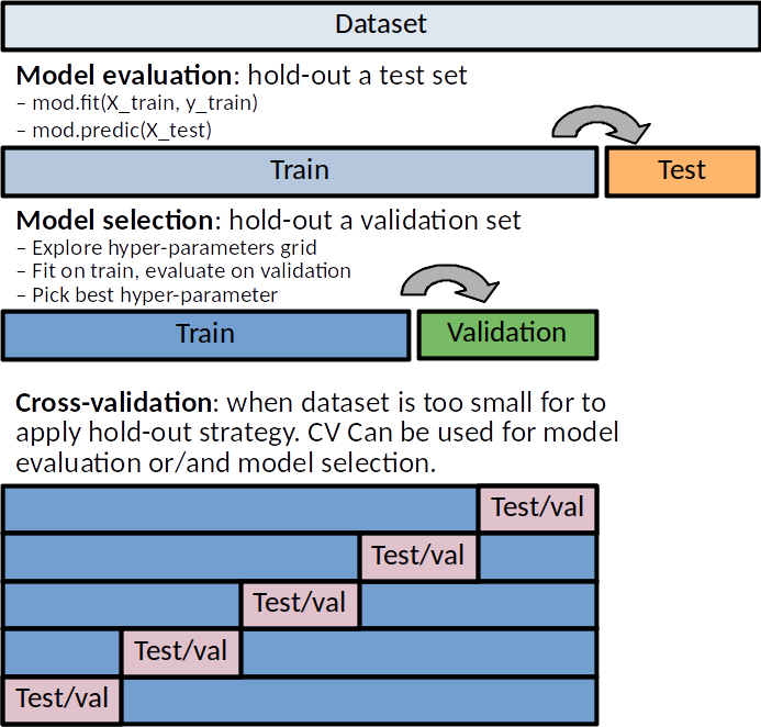
Train, validation and test sets

Machine learning algorithms tend to overfit training data. Predictive performances MUST be evaluated on independant hold-out dataset. A split of into a training test and an independent test set mandatory. However to set the hyperparameters the dataset is generally splitted into three sets:

1. Training Set (Fitting the Model and Learning Parameters)

• The training set is used to fit the model by learning its parameters (e.g., weights in a neural network, coefficients in a regression model).

• The algorithm adjusts its parameters to minimize a chosen loss function (e.g., MSE for regression, cross-entropy for classification).

• The model learns patterns from this data, but using only the training set risks overfitting—where the model memorizes data instead of generalizing.

• Role: Learn the parameters of the model.

2. Validation Set (Hyperparameter Tuning and Model Selection)

• The validation set is used to fine-tune the model’s hyperparameters (e.g., learning rate, number of layers, number of clusters).

• Hyperparameters are not directly learned from data but are instead set before training.

• The validation set helps to assess different model configurations, preventing overfitting by ensuring that the model generalizes beyond the training set.

• If we see high performance on the training set but poor performance on the validation set, we are likely overfitting.

• The process of choosing the best hyperparameters based on the validation set is called model selection.

• Role: Tune hyperparameters and select the best model configuration.

• Data Leakage Risk: If we tune hyperparameters too much on the validation set, it essentially becomes part of training, leading to potential overfitting on it.

3. Test Set (Final Independent Evaluation)

• The test set is an independent dataset used to evaluate the final model after training and hyperparameter tuning.

• This provides an unbiased estimate of how the model will perform on completely new data.

• The model should never be trained or tuned using the test set to ensure a fair evaluation.

• Performance metrics (e.g., accuracy, F1-score, ROC-AUC) on the test set indicate how well the model is expected to perform in real-world scenarios.

• Role: Evaluate the final model’s performance on unseen data.

Summary:

• Training set

  • Fits model parameters.

  • High risk of overfitting if the model is too complex.

• Validation set

  • Tunes hyperparameters and selects the best model.

  • Risk of of overfitting if tuning too much.

• Test set

  • Provides a final evaluation on unseen data.

Split dataset in train/test sets to train and assess the the final model after training and hyperparameter tuning.

X_train, X_test, y_train, y_test =\
    train_test_split(X, y, test_size=0.25, shuffle=True, random_state=42)

mod = lm.Ridge(alpha=10)

mod.fit(X_train, y_train)

y_pred_test = mod.predict(X_test)
print("Test R2: %.2f" % metrics.r2_score(y_test, y_pred_test))

Test R2: 0.74

Cross-Validation (CV)

If sample size is limited, train/validation/test split may be impossible:

• Large training+validation set (80%) small test set (20%) might provide a poor estimation of the predictive performances on few test samples. The same argument stands for train vs validation samples.

• On the contrary, large test set and small training set might produce a poorly estimated learner.

Cross Validation (CV) (Scikit-learn)can be used to replace train/validation split and/or train+validation / test split. Main procedure:

1. The dataset is divided into k equal-sized subsets (folds).

2. The model is trained k times, each time using k-1 folds as the training set and 1 fold as the validation set.

3. The final performance is the average of the k validation scores.

For 10-fold we can either average over 10 values (Macro measure) or concatenate the 10 experiments and compute the micro measures.

Two strategies [micro vs macro estimates](https://stats.stackexchange.com/questions/34611/meanscores-vs-scoreconcatenation-in-cross-validation):

• Micro measure: average(individual scores): compute a score \(\mathcal{S}\) for each sample and average over all samples. It is similar to average score(concatenation): an averaged score computed over all concatenated samples.

• Macro measure mean(CV scores) (the most commonly used method): compute a score \(\mathcal{S}\) on each each fold k and average across folds:

These two measures (an average of average vs. a global average) are generally similar. They may differ slightly is folds are of different sizes. This validation scheme is known as the K-Fold CV. Typical choices of K are 5 or 10, [Kohavi 1995]. The extreme case where K = N is known as Leave-One-Out Cross-Validation, LOO-CV.

CV for regression

Usually the error function \(\mathcal{L}()\) is the r-squared score. However other function (MAE, MSE) can be used.

CV with explicit loop:

estimator = lm.Ridge(alpha=10)

cv = KFold(n_splits=5, shuffle=True, random_state=42)
r2_train, r2_test = list(), list()

for train, test in cv.split(X):
    estimator.fit(X[train, :], y[train])
    r2_train.append(metrics.r2_score(y[train], estimator.predict(X[train, :])))
    r2_test.append(metrics.r2_score(y[test], estimator.predict(X[test, :])))

print("Train r2:%.2f" % np.mean(r2_train))
print("Test  r2:%.2f" % np.mean(r2_test))

Train r2:0.99
Test  r2:0.67

Scikit-learn provides user-friendly function to perform CV

cross_val_score: single metric

scores = cross_val_score(estimator=estimator, X=X, y=y, cv=5)
print("Test  r2:%.2f" % scores.mean())

cv = KFold(n_splits=5, shuffle=True, random_state=42)
scores = cross_val_score(estimator=estimator, X=X, y=y, cv=cv)
print("Test  r2:%.2f" % scores.mean())

Test  r2:0.73
Test  r2:0.67

cross_validate: multi metric, + time, etc.

scores = cross_validate(estimator=mod, X=X, y=y, cv=cv,
                        scoring=['r2', 'neg_mean_absolute_error'])

print("Test R2:%.2f; MAE:%.2f" % (scores['test_r2'].mean(),
                                  -scores['test_neg_mean_absolute_error'].mean()))

Test R2:0.67; MAE:55.27

CV for classification: stratify for the target label

With classification problems it is essential to sample folds where each set contains approximately the same percentage of samples of each target class as the complete set. This is called stratification. In this case, we will use StratifiedKFold with is a variation of k-fold which returns stratified folds. As error function we recommend:

• The balanced accuracy

• The ROC-AUC

CV with explicit loop:

X, y = datasets.make_classification(n_samples=100, n_features=100, shuffle=True,
                                    n_informative=10, random_state=42)

mod = lm.LogisticRegression(C=1, solver='lbfgs')

cv = StratifiedKFold(n_splits=5)

# Lists to store scores by folds (for macro measure only)
bacc, auc = [], []

for train, test in cv.split(X, y):
    mod.fit(X[train, :], y[train])
    bacc.append(metrics.roc_auc_score(
        y[test], mod.decision_function(X[test, :])))
    auc.append(metrics.balanced_accuracy_score(
        y[test], mod.predict(X[test, :])))

print("Test AUC:%.2f; bACC:%.2f" % (np.mean(bacc), np.mean(auc)))

Test AUC:0.86; bACC:0.79

cross_val_score: single metric

scores = cross_val_score(estimator=mod, X=X, y=y, cv=5)

print("Test  ACC:%.2f" % scores.mean())

Test  ACC:0.79

Provide your own CV and score

def balanced_acc(estimator, X, y, **kwargs):
    """Balanced acuracy scorer."""
    return metrics.recall_score(y, estimator.predict(X), average=None).mean()


scores = cross_val_score(estimator=mod, X=X, y=y, cv=cv,
                         scoring=balanced_acc)
print("Test  bACC:%.2f" % scores.mean())

Test  bACC:0.79

cross_validate: multi metric, + time, etc.

scores = cross_validate(estimator=mod, X=X, y=y, cv=cv,
                        scoring=['balanced_accuracy', 'roc_auc'])

print("Test AUC:%.2f; bACC:%.2f" % (scores['test_roc_auc'].mean(),
                                    scores['test_balanced_accuracy'].mean()))

Test AUC:0.86; bACC:0.79

Cross-validation for model selection (GridSearchCV)

Combine CV and grid search: GridSearchCV perform hyperparameter tuning (model selection) by systematically searching the best combination of hyperparameters evaluating all possible combinations (over a grid of possible values) using cross-validation:

1. Define the model: Choose a machine learning model (e.g., SVM, Random Forest).

2. Specify hyperparameters: Create a dictionary of hyperparameters and their possible values.

3. Perform exhaustive search: GridSearchCV trains the model with every possible combination of hyperparameters.

4. Cross-validation: For each combination, it uses k-fold cross-validation (default cv=5).

5. Select the best model: The combination with the highest validation performance is chosen. By default, refit an estimator using the best found parameters on the whole dataset.

# Outer, tain/test, split:
X_train, X_test, y_train, y_test =\
    train_test_split(X, y, test_size=0.25, shuffle=True, random_state=42)

cv_inner = StratifiedKFold(n_splits=5, shuffle=True, random_state=42)

# Inner Cross-Validation (tain/validation, splits) for model selection
lm_cv = GridSearchCV(lm.LogisticRegression(), {'C': 10. ** np.arange(-3, 3)},
                     cv=cv_inner, n_jobs=5)

# Fit, including model selection with internal CV
lm_cv.fit(X_train, y_train)

# Predict
y_pred_test = lm_cv.predict(X_test)
print("Test bACC: %.2f" % metrics.balanced_accuracy_score(y_test, y_pred_test))

Test bACC: 0.75

Cross-validation for both model (outer) evaluation and model (inner) selection

cv_outer = StratifiedKFold(n_splits=5, shuffle=True, random_state=42)
cv_inner = StratifiedKFold(n_splits=5, shuffle=True, random_state=42)

# Cross-validation for model (inner) selection
lm_cv = GridSearchCV(lm.Ridge(), {'alpha': 10. ** np.arange(-3, 3)},
                     cv=cv_inner, n_jobs=5)

# Cross-validation for model (outer) evaluation
scores = cross_validate(estimator=mod, X=X, y=y, cv=cv_outer,
                        scoring=['balanced_accuracy', 'roc_auc'])

print("Test AUC:%.2f; bACC:%.2f, Time: %.2fs" % (scores['test_roc_auc'].mean(),
                                                 scores['test_balanced_accuracy'].mean(
),
    scores['fit_time'].sum()))

Test AUC:0.85; bACC:0.74, Time: 0.01s

Models with built-in cross-validation

Let sklearn select the best parameters over a default grid.

Classification

print("== Logistic Ridge (L2 penalty) ==")
mod_cv = lm.LogisticRegressionCV(class_weight='balanced',
                                 scoring='balanced_accuracy',
                                 n_jobs=-1, cv=5)
scores = cross_val_score(estimator=mod_cv, X=X, y=y, cv=5)
print("Test  ACC:%.2f" % scores.mean())

== Logistic Ridge (L2 penalty) ==
Test  ACC:0.79

Regression

X, y, coef = datasets.make_regression(n_samples=50, n_features=100, noise=10,
                                      n_informative=2, random_state=42, coef=True)

print("== Ridge (L2 penalty) ==")
model = lm.RidgeCV(cv=3)
scores = cross_val_score(estimator=model, X=X, y=y, cv=5)
print("Test  r2:%.2f" % scores.mean())

print("== Lasso (L1 penalty) ==")
model = lm.LassoCV(n_jobs=-1, cv=3)
scores = cross_val_score(estimator=model, X=X, y=y, cv=5)
print("Test  r2:%.2f" % scores.mean())

print("== ElasticNet (L1 penalty) ==")
model = lm.ElasticNetCV(l1_ratio=[.1, .5, .9], n_jobs=-1, cv=3)
scores = cross_val_score(estimator=model, X=X, y=y, cv=5)
print("Test  r2:%.2f" % scores.mean())

== Ridge (L2 penalty) ==
Test  r2:0.16
== Lasso (L1 penalty) ==
Test  r2:0.74
== ElasticNet (L1 penalty) ==
Test  r2:0.58

Random Permutations: sample the null distribution

A permutation test is a type of non-parametric randomization test in which the null distribution of a test statistic is estimated by randomly permuting the observations.

Permutation tests are highly attractive because they make no assumptions other than that the observations are independent and identically distributed under the null hypothesis.

1. Compute a observed statistic \(t_{obs}\) on the data.

2. Use randomization to compute the distribution of \(t\) under the null hypothesis: Perform \(N\) random permutation of the data. For each sample of permuted data, \(i\) the data compute the statistic \(t_i\). This procedure provides the distribution of t under the null hypothesis \(H_0\): \(P(t \vert H_0)\)

3. Compute the p-value = \(P(t>t_{obs} | H_0) \left\vert\{t_i > t_{obs}\}\right\vert\), where \(t_i's include :math:`t_{obs}\).

Example Ridge regression

Sample the distributions of r-squared and coefficients of ridge regression under the null hypothesis. Simulated dataset:

# Regression dataset where first two features are predictive
np.random.seed(0)
n_features = 5
n_features_info = 2
n_samples = 100
X = np.random.randn(100, 5)
beta = np.zeros(n_features)
beta[:n_features_info] = 1
Xbeta = np.dot(X, beta)
eps = np.random.randn(n_samples)
y = Xbeta + eps


# Fit model on all data (!! risk of overfit)
model = lm.RidgeCV()
model.fit(X, y)
print("Coefficients on all data:")
print(model.coef_)

# Random permutation loop
nperm = 1000  # !! Should be at least 1000 (to assess a p-value at 1%)
scores_names = ["r2"]
scores_perm = np.zeros((nperm + 1, len(scores_names)))
coefs_perm = np.zeros((nperm + 1, X.shape[1]))

scores_perm[0, :] = metrics.r2_score(y, model.predict(X))
coefs_perm[0, :] = model.coef_

orig_all = np.arange(X.shape[0])
for perm_i in range(1, nperm + 1):
    model.fit(X, np.random.permutation(y))
    y_pred = model.predict(X).ravel()
    scores_perm[perm_i, :] = metrics.r2_score(y, y_pred)
    coefs_perm[perm_i, :] = model.coef_

# One-tailed empirical p-value
pval_pred_perm = np.sum(scores_perm >= scores_perm[0]) / scores_perm.shape[0]
pval_coef_perm = np.sum(
    coefs_perm >= coefs_perm[0, :], axis=0) / coefs_perm.shape[0]

print("R2 p-value: %.3f" % pval_pred_perm)
print("Coeficients p-values:", np.round(pval_coef_perm, 3))

Coefficients on all data:
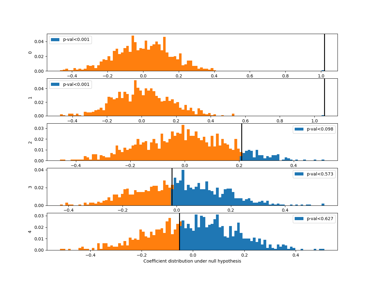
[ 1.01872179  1.05713711  0.20873888 -0.01784094 -0.05265821]
R2 p-value: 0.001
Coeficients p-values: [0.001 0.001 0.098 0.573 0.627]

Compute p-values corrected for multiple comparisons using FWER max-T (Westfall and Young, 1993) procedure.

pval_coef_perm_tmax = np.array([np.sum(coefs_perm.max(axis=1) >= coefs_perm[0, j])
                                for j in range(coefs_perm.shape[1])]) / coefs_perm.shape[0]
print("P-values with FWER (Westfall and Young) correction")
print(pval_coef_perm_tmax)

P-values with FWER (Westfall and Young) correction
[0.000999   0.000999   0.41058941 0.98001998 0.99200799]

Plot distribution of third coefficient under null-hypothesis Coeffitients 0 and 1 are significantly different from 0.

def hist_pvalue(perms, ax, name):
    """Plot statistic distribution as histogram.

    Paramters
    ---------
    perms: 1d array, statistics under the null hypothesis.
           perms[0] is the true statistic .
    """
    # Re-weight to obtain distribution
    pval = np.sum(perms >= perms[0]) / perms.shape[0]
    weights = np.ones(perms.shape[0]) / perms.shape[0]
    ax.hist([perms[perms >= perms[0]], perms], histtype='stepfilled',
            bins=100, label="p-val<%.3f" % pval,
            weights=[weights[perms >= perms[0]], weights])
    # , label="observed statistic")
    ax.axvline(x=perms[0], color="k", linewidth=2)
    ax.set_ylabel(name)
    ax.legend()
    return ax


n_coef = coefs_perm.shape[1]
fig, axes = plt.subplots(n_coef, 1, figsize=(12, 9))
for i in range(n_coef):
    hist_pvalue(coefs_perm[:, i], axes[i], str(i))

_ = axes[-1].set_xlabel("Coefficient distribution under null hypothesis")

Exercise

Given the logistic regression presented above and its validation given a 5 folds CV.

1. Compute the p-value associated with the prediction accuracy measured with 5CV using a permutation test.

2. Compute the p-value associated with the prediction accuracy using a parametric test.

Bootstrapping

Bootstrapping is a statistical technique which consists in generating sample (called bootstrap samples) from an initial dataset of size N by randomly drawing with replacement N observations. It provides sub-samples with the same distribution than the original dataset. It aims to:

1. Assess the variability (standard error, Confidence Intervals (CI) of performances scores or estimated parameters (see Efron et al. 1986).

2. Regularize model by fitting several models on bootstrap samples and averaging their predictions (see Baging and random-forest).

A great advantage of bootstrap is its simplicity. It is a straightforward way to derive estimates of standard errors and confidence intervals for complex estimators of complex parameters of the distribution, such as percentile points, proportions, odds ratio, and correlation coefficients.

1. Perform \(B\) sampling, with replacement, of the dataset.

2. For each sample \(i\) fit the model and compute the scores.

3. Assess standard errors and confidence intervals of scores using the scores obtained on the \(B\) resampled dataset. Or, average models predictions.

References:

[Efron B, Tibshirani R. Bootstrap methods for standard errors, confidence intervals, and other measures of statistical accuracy. Stat Sci 1986;1:54–75](https://projecteuclid.org/download/pdf_1/euclid.ss/1177013815)

# Bootstrap loop
nboot = 100  # !! Should be at least 1000
scores_names = ["r2"]
scores_boot = np.zeros((nboot, len(scores_names)))
coefs_boot = np.zeros((nboot, X.shape[1]))

orig_all = np.arange(X.shape[0])
for boot_i in range(nboot):
    boot_tr = np.random.choice(orig_all, size=len(orig_all), replace=True)
    boot_te = np.setdiff1d(orig_all, boot_tr, assume_unique=False)
    Xtr, ytr = X[boot_tr, :], y[boot_tr]
    Xte, yte = X[boot_te, :], y[boot_te]
    model.fit(Xtr, ytr)
    y_pred = model.predict(Xte).ravel()
    scores_boot[boot_i, :] = metrics.r2_score(yte, y_pred)
    coefs_boot[boot_i, :] = model.coef_

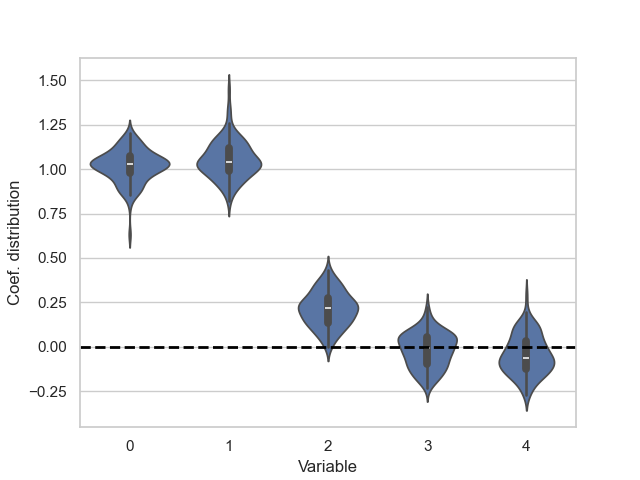
Compute Mean, SE, CI Coeffitients 0 and 1 are significantly different from 0.

scores_boot = pd.DataFrame(scores_boot, columns=scores_names)
scores_stat = scores_boot.describe(percentiles=[.975, .5, .025])

print("r-squared: Mean=%.2f, SE=%.2f, CI=(%.2f %.2f)" %
      tuple(scores_stat.loc[["mean", "std", "2.5%", "97.5%"], "r2"]))

coefs_boot = pd.DataFrame(coefs_boot)
coefs_stat = coefs_boot.describe(percentiles=[.975, .5, .025])
print("Coefficients distribution")
print(coefs_stat)

r-squared: Mean=0.59, SE=0.09, CI=(0.40 0.73)
Coefficients distribution
                0           1           2           3           4
count  100.000000  100.000000  100.000000  100.000000  100.000000
mean     1.017598    1.053832    0.212464   -0.018828   -0.045851
std      0.091508    0.105196    0.097532    0.097343    0.110555
min      0.631917    0.819190   -0.002689   -0.231580   -0.270810
2.5%     0.857418    0.883319    0.032672   -0.195018   -0.233241
50%      1.027161    1.038053    0.216531   -0.010023   -0.063331
97.5%    1.174707    1.289990    0.392701    0.150340    0.141587
max      1.204006    1.449672    0.432764    0.220711    0.290928

Plot coefficient distribution

df = pd.DataFrame(coefs_boot)
staked = pd.melt(df, var_name="Variable", value_name="Coef. distribution")
sns.set_theme(style="whitegrid")
ax = sns.violinplot(x="Variable", y="Coef. distribution", data=staked)
_ = ax.axhline(0, ls='--', lw=2, color="black")

Parallel Computation

Dataset

X, y = datasets.make_classification(
    n_samples=20, n_features=5, n_informative=2, random_state=42)
cv = StratifiedKFold(n_splits=5)

Classic sequential computation of CV:

estimator = lm.LogisticRegression(C=1, solver='lbfgs')
y_test_pred_seq = np.zeros(len(y))  # Store predictions in the original order
coefs_seq = list()
for train, test in cv.split(X, y):
    X_train, X_test, y_train, y_test = X[train,
                                         :], X[test, :], y[train], y[test]
    estimator.fit(X_train, y_train)
    y_test_pred_seq[test] = estimator.predict(X_test)
    coefs_seq.append(estimator.coef_)

test_accs = [metrics.accuracy_score(
    y[test], y_test_pred_seq[test]) for train, test in cv.split(X, y)]

# Accuracy
print(np.mean(test_accs), test_accs)

# Coef
coefs_cv = np.array(coefs_seq)
print("Mean of the coef")
print(coefs_cv.mean(axis=0).round(2))
print("Std Err of the coef")
print((coefs_cv.std(axis=0) / np.sqrt(coefs_cv.shape[0])).round(2))

0.8 [0.5, 0.5, 1.0, 1.0, 1.0]
Mean of the coef
[[-0.87  0.56  1.11 -0.08 -0.32]]
Std Err of the coef
[[0.03 0.02 0.02 0.09 0.03]]

Parallelization using cross_validate function

estimator = lm.LogisticRegression(C=1, solver='lbfgs')
cv_results = cross_validate(estimator, X, y, cv=cv, n_jobs=5)
print(np.mean(cv_results['test_score']), cv_results['test_score'])

0.8 [0.5 0.5 1.  1.  1. ]

Parallel computation with joblib:

def _split_fit_predict(estimator, X, y, train, test):
    X_train, X_test, y_train, y_test = X[train,
                                         :], X[test, :], y[train], y[test]
    estimator.fit(X_train, y_train)
    return [estimator.predict(X_test), estimator.coef_]


estimator = lm.LogisticRegression(C=1, solver='lbfgs')

parallel = Parallel(n_jobs=5)
cv_ret = parallel(
    delayed(_split_fit_predict)(
        clone(estimator), X, y, train, test)
    for train, test in cv.split(X, y))

y_test_pred_cv, coefs_cv = zip(*cv_ret)

y_test_pred = np.zeros(len(y))
for i, (train, test) in enumerate(cv.split(X, y)):
    y_test_pred[test] = y_test_pred_cv[i]

test_accs = [metrics.accuracy_score(
    y[test], y_test_pred[test]) for train, test in cv.split(X, y)]
print(np.mean(test_accs), test_accs)

0.8 [0.5, 0.5, 1.0, 1.0, 1.0]

Test same predictions and same coefficients

assert np.all(y_test_pred == y_test_pred_seq)
assert np.allclose(np.array(coefs_cv).squeeze(), np.array(coefs_seq).squeeze())