Note
Go to the end to download the full example code.
Hands-On: Brain volumes study
The study provides the brain volumes of grey matter (gm), white matter (wm) and cerebrospinal fluid) (csf) of 808 anatomical MRI scans.
import os
import tempfile
import urllib.request

import pandas as pd

# Stat
import statsmodels.formula.api as smfrmla
import statsmodels.api as sm
import scipy.stats

# Plot
import matplotlib.pyplot as plt
import seaborn as sns

# Plot parameters
plt.style.use('seaborn-v0_8-whitegrid')
fig_w, fig_h = plt.rcParams.get('figure.figsize')
plt.rcParams['figure.figsize'] = (fig_w, fig_h * .5)
Manipulate data
Set the working directory within a directory called “brainvol”
Create 2 subdirectories: data that will contain downloaded data and reports for results of the analysis.
WD = os.path.join(tempfile.gettempdir(), "brainvol")
os.makedirs(WD, exist_ok=True)
#os.chdir(WD)

# use cookiecutter file organization
# https://drivendata.github.io/cookiecutter-data-science/
os.makedirs(os.path.join(WD, "data"), exist_ok=True)
#os.makedirs("reports", exist_ok=True)
Fetch data
Demographic data demo.csv (columns: participant_id, site, group, age, sex) and tissue volume data: group is Control or Patient. site is the recruiting site.
Gray matter volume gm.csv (columns: participant_id, session, gm_vol)
White matter volume wm.csv (columns: participant_id, session, wm_vol)
Cerebrospinal Fluid csf.csv (columns: participant_id, session, csf_vol)
base_url = 'https://github.com/duchesnay/pystatsml/raw/master/datasets/brain_volumes/%s'
data = dict()
for file in ["demo.csv", "gm.csv", "wm.csv", "csf.csv"]:
    urllib.request.urlretrieve(base_url % file, os.path.join(WD, "data", file))

# Read all CSV in one line
# dicts = {k: pd.read_csv(os.path.join(WD, "data", "%s.csv" % k))
#          for k in ["demo", "gm", "wm", "csf"]}

demo = pd.read_csv(os.path.join(WD, "data", "demo.csv"))
gm = pd.read_csv(os.path.join(WD, "data", "gm.csv"))
wm = pd.read_csv(os.path.join(WD, "data", "wm.csv"))
csf = pd.read_csv(os.path.join(WD, "data", "csf.csv"))

print("tables can be merge using shared columns")
print(gm.head())
tables can be merge using shared columns
  participant_id session    gm_vol
0    sub-S1-0002  ses-01  0.672506
1    sub-S1-0002  ses-02  0.678772
2    sub-S1-0002  ses-03  0.665592
3    sub-S1-0004  ses-01  0.890714
4    sub-S1-0004  ses-02  0.881127
Merge tables according to participant_id
brain_vol = pd.merge(pd.merge(pd.merge(demo, gm), wm), csf)
assert brain_vol.shape == (808, 9)
Drop rows with missing values
brain_vol = brain_vol.dropna()
assert brain_vol.shape == (766, 9)
Compute Total Intra-cranial volume tiv_vol = gm_vol + csf_vol + wm_vol.
brain_vol["tiv_vol"] = brain_vol["gm_vol"] + \
    brain_vol["wm_vol"] + brain_vol["csf_vol"]
Compute tissue fractions gm_f = gm_vol / tiv_vol, wm_f = wm_vol / tiv_vol.
brain_vol["gm_f"] = brain_vol["gm_vol"] / brain_vol["tiv_vol"]
brain_vol["wm_f"] = brain_vol["wm_vol"] / brain_vol["tiv_vol"]
Save in a excel file brain_vol.xlsx
brain_vol.to_excel(os.path.join(WD, "data", "brain_vol.xlsx"),
                   sheet_name='data', index=False)
Descriptive Statistics
Load excel file brain_vol.xlsx
brain_vol = pd.read_excel(os.path.join(WD, "data", "brain_vol.xlsx"),
                          sheet_name='data')
# Round float at 2 decimals when printing
pd.options.display.float_format = '{:,.2f}'.format
Descriptive statistics Most of participants have several MRI sessions (column session) Select on rows from session one “ses-01”
brain_vol1 = brain_vol[brain_vol.session == "ses-01"]
# Check that there are no duplicates
assert len(brain_vol1.participant_id.unique()) == len(brain_vol1.participant_id)
Global descriptives statistics of numerical variables
desc_glob_num = brain_vol1.describe()
print(desc_glob_num)
         age  gm_vol  wm_vol  csf_vol  tiv_vol   gm_f   wm_f
count 244.00  244.00  244.00   244.00   244.00 244.00 244.00
mean   34.54    0.71    0.44     0.31     1.46   0.49   0.30
std    12.09    0.08    0.07     0.08     0.17   0.04   0.03
min    18.00    0.48    0.05     0.12     0.83   0.37   0.06
25%    25.00    0.66    0.40     0.25     1.34   0.46   0.28
50%    31.00    0.70    0.43     0.30     1.45   0.49   0.30
75%    44.00    0.77    0.48     0.37     1.57   0.52   0.31
max    61.00    1.03    0.62     0.63     2.06   0.60   0.36
Global Descriptive statistics of categorical variable
desc_glob_cat = brain_vol1[["site", "group", "sex"]].describe(include='all')
print(desc_glob_cat)

print("Get count by level")
desc_glob_cat = pd.DataFrame({col: brain_vol1[col].value_counts().to_dict()
                             for col in ["site", "group", "sex"]})
print(desc_glob_cat)
       site    group  sex
count   244      244  244
unique    7        2    2
top      S7  Patient    M
freq     65      157  155
Get count by level
         site  group    sex
S7      65.00    NaN    NaN
S5      62.00    NaN    NaN
S8      59.00    NaN    NaN
S3      29.00    NaN    NaN
S4      15.00    NaN    NaN
S1      13.00    NaN    NaN
S6       1.00    NaN    NaN
Patient   NaN 157.00    NaN
Control   NaN  87.00    NaN
M         NaN    NaN 155.00
F         NaN    NaN  89.00
Remove the single participant from site 6
brain_vol = brain_vol[brain_vol.site != "S6"]
brain_vol1 = brain_vol[brain_vol.session == "ses-01"]
desc_glob_cat = pd.DataFrame({col: brain_vol1[col].value_counts().to_dict()
                             for col in ["site", "group", "sex"]})
print(desc_glob_cat)
         site  group    sex
S7      65.00    NaN    NaN
S5      62.00    NaN    NaN
S8      59.00    NaN    NaN
S3      29.00    NaN    NaN
S4      15.00    NaN    NaN
S1      13.00    NaN    NaN
Patient   NaN 157.00    NaN
Control   NaN  86.00    NaN
M         NaN    NaN 155.00
F         NaN    NaN  88.00
Descriptives statistics of numerical variables per clinical status
desc_group_num = brain_vol1[["group", 'gm_vol']].groupby("group").describe()
print(desc_group_num)
        gm_vol
         count mean  std  min  25%  50%  75%  max
group
Control  86.00 0.72 0.09 0.48 0.66 0.71 0.78 1.03
Patient 157.00 0.70 0.08 0.53 0.65 0.70 0.76 0.90
Statistics
Objectives:
Site effect of gray matter atrophy
Test the association between the age and gray matter atrophy in the control and patient population independently.
Test for differences of atrophy between the patients and the controls
Test for interaction between age and clinical status, ie: is the brain atrophy process in patient population faster than in the control population.
The effect of the medication in the patient population.
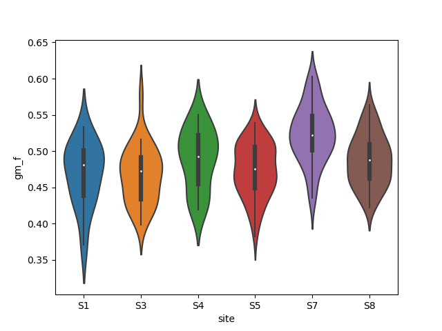
1 Site effect on Grey Matter atrophy
The model is Oneway Anova gm_f ~ site The ANOVA test has important assumptions that must be satisfied in order for the associated p-value to be valid.
The samples are independent.
Each sample is from a normally distributed population.
The population standard deviations of the groups are all equal. This property is known as homoscedasticity.
Plot
sns.violinplot(x="site", y="gm_f", data=brain_vol1)
# sns.violinplot(x="site", y="wm_f", data=brain_vol1)

brain_vol1.groupby('site')['age'].describe()
Stats with scipy
fstat, pval = scipy.stats.f_oneway(*[brain_vol1.gm_f[brain_vol1.site == s]
                                   for s in brain_vol1.site.unique()])
print("Oneway Anova gm_f ~ site F=%.2f, p-value=%E" % (fstat, pval))
Oneway Anova gm_f ~ site F=14.82, p-value=1.188136E-12
Stats with statsmodels
anova = smfrmla.ols("gm_f ~ site", data=brain_vol1).fit()
# print(anova.summary())
print("Site explains %.2f%% of the grey matter fraction variance" %
      (anova.rsquared * 100))

print(sm.stats.anova_lm(anova, typ=2))
Site explains 23.82% of the grey matter fraction variance
          sum_sq     df     F  PR(>F)
site        0.11   5.00 14.82    0.00
Residual    0.35 237.00   NaN     NaN
2. Test the association between the age and gray matter atrophy in the control and patient population independently.
Plot
sns.lmplot(x="age", y="gm_f", hue="group", data=brain_vol1)

brain_vol1_ctl = brain_vol1[brain_vol1.group == "Control"]
brain_vol1_pat = brain_vol1[brain_vol1.group == "Patient"]
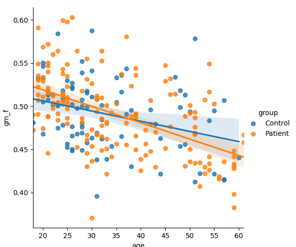
Stats with scipy
print("--- In control population ---")
beta, beta0, r_value, p_value, std_err = \
    scipy.stats.linregress(x=brain_vol1_ctl.age, y=brain_vol1_ctl.gm_f)

print("gm_f = %f * age + %f" % (beta, beta0))
print("Corr: %f, r-squared: %f, p-value: %f, std_err: %f"\
      % (r_value, r_value**2, p_value, std_err))

print("--- In patient population ---")
beta, beta0, r_value, p_value, std_err = \
    scipy.stats.linregress(x=brain_vol1_pat.age, y=brain_vol1_pat.gm_f)

print("gm_f = %f * age + %f" % (beta, beta0))
print("Corr: %f, r-squared: %f, p-value: %f, std_err: %f"\
      % (r_value, r_value**2, p_value, std_err))

print("Decrease seems faster in patient than in control population")
--- In control population ---
gm_f = -0.001181 * age + 0.529829
Corr: -0.325122, r-squared: 0.105704, p-value: 0.002255, std_err: 0.000375
--- In patient population ---
gm_f = -0.001899 * age + 0.556886
Corr: -0.528765, r-squared: 0.279592, p-value: 0.000000, std_err: 0.000245
Decrease seems faster in patient than in control population
Stats with statsmodels
print("--- In control population ---")
lr = smfrmla.ols("gm_f ~ age", data=brain_vol1_ctl).fit()
print(lr.summary())
print("Age explains %.2f%% of the grey matter fraction variance" %
      (lr.rsquared * 100))

print("--- In patient population ---")
lr = smfrmla.ols("gm_f ~ age", data=brain_vol1_pat).fit()
print(lr.summary())
print("Age explains %.2f%% of the grey matter fraction variance" %
      (lr.rsquared * 100))
--- In control population ---
                            OLS Regression Results
==============================================================================
Dep. Variable:                   gm_f   R-squared:                       0.106
Model:                            OLS   Adj. R-squared:                  0.095
Method:                 Least Squares   F-statistic:                     9.929
Date:               jeu., 08 mai 2025   Prob (F-statistic):            0.00226
Time:                        02:16:34   Log-Likelihood:                 159.34
No. Observations:                  86   AIC:                            -314.7
Df Residuals:                      84   BIC:                            -309.8
Df Model:                           1
Covariance Type:            nonrobust
==============================================================================
                 coef    std err          t      P>|t|      [0.025      0.975]
------------------------------------------------------------------------------
Intercept      0.5298      0.013     40.350      0.000       0.504       0.556
age           -0.0012      0.000     -3.151      0.002      -0.002      -0.000
==============================================================================
Omnibus:                        0.946   Durbin-Watson:                   1.628
Prob(Omnibus):                  0.623   Jarque-Bera (JB):                0.782
Skew:                           0.233   Prob(JB):                        0.676
Kurtosis:                       2.962   Cond. No.                         111.
==============================================================================

Notes:
[1] Standard Errors assume that the covariance matrix of the errors is correctly specified.
Age explains 10.57% of the grey matter fraction variance
--- In patient population ---
                            OLS Regression Results
==============================================================================
Dep. Variable:                   gm_f   R-squared:                       0.280
Model:                            OLS   Adj. R-squared:                  0.275
Method:                 Least Squares   F-statistic:                     60.16
Date:               jeu., 08 mai 2025   Prob (F-statistic):           1.09e-12
Time:                        02:16:34   Log-Likelihood:                 289.38
No. Observations:                 157   AIC:                            -574.8
Df Residuals:                     155   BIC:                            -568.7
Df Model:                           1
Covariance Type:            nonrobust
==============================================================================
                 coef    std err          t      P>|t|      [0.025      0.975]
------------------------------------------------------------------------------
Intercept      0.5569      0.009     60.817      0.000       0.539       0.575
age           -0.0019      0.000     -7.756      0.000      -0.002      -0.001
==============================================================================
Omnibus:                        2.310   Durbin-Watson:                   1.325
Prob(Omnibus):                  0.315   Jarque-Bera (JB):                1.854
Skew:                           0.230   Prob(JB):                        0.396
Kurtosis:                       3.268   Cond. No.                         111.
==============================================================================

Notes:
[1] Standard Errors assume that the covariance matrix of the errors is correctly specified.
Age explains 27.96% of the grey matter fraction variance
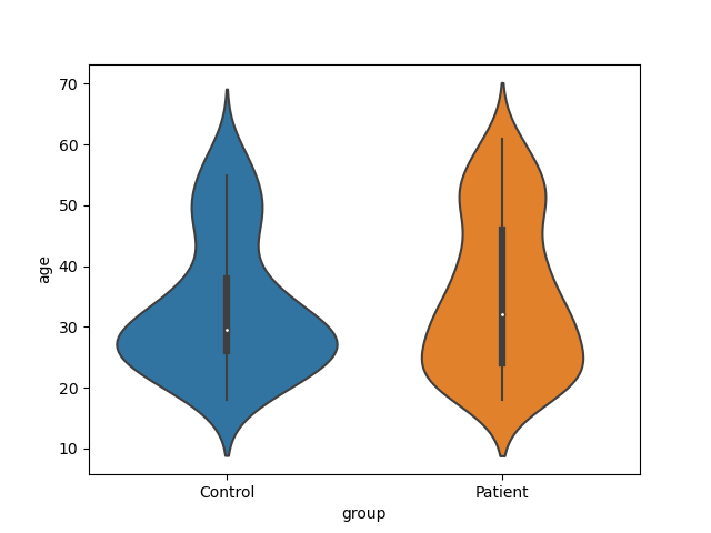
Before testing for differences of atrophy between the patients ans the controls Preliminary tests for age x group effect (patients would be older or younger than Controls)
Plot
sns.violinplot(x="group", y="age", data=brain_vol1)
<Axes: xlabel='group', ylabel='age'>
Stats with scipy
print(scipy.stats.ttest_ind(brain_vol1_ctl.age, brain_vol1_pat.age))
TtestResult(statistic=np.float64(-1.2155557697674162), pvalue=np.float64(0.225343592508479), df=np.float64(241.0))
Stats with statsmodels
print(smfrmla.ols("age ~ group", data=brain_vol1).fit().summary())
print("No significant difference in age between patients and controls")
                            OLS Regression Results
==============================================================================
Dep. Variable:                    age   R-squared:                       0.006
Model:                            OLS   Adj. R-squared:                  0.002
Method:                 Least Squares   F-statistic:                     1.478
Date:               jeu., 08 mai 2025   Prob (F-statistic):              0.225
Time:                        02:16:34   Log-Likelihood:                -949.69
No. Observations:                 243   AIC:                             1903.
Df Residuals:                     241   BIC:                             1910.
Df Model:                           1
Covariance Type:            nonrobust
====================================================================================
                       coef    std err          t      P>|t|      [0.025      0.975]
------------------------------------------------------------------------------------
Intercept           33.2558      1.305     25.484      0.000      30.685      35.826
group[T.Patient]     1.9735      1.624      1.216      0.225      -1.225       5.172
==============================================================================
Omnibus:                       35.711   Durbin-Watson:                   2.096
Prob(Omnibus):                  0.000   Jarque-Bera (JB):               20.726
Skew:                           0.569   Prob(JB):                     3.16e-05
Kurtosis:                       2.133   Cond. No.                         3.12
==============================================================================

Notes:
[1] Standard Errors assume that the covariance matrix of the errors is correctly specified.
No significant difference in age between patients and controls
Preliminary tests for sex x group (more/less males in patients than in Controls)
crosstab = pd.crosstab(brain_vol1.sex, brain_vol1.group)
print("Obeserved contingency table")
print(crosstab)

chi2, pval, dof, expected = scipy.stats.chi2_contingency(crosstab)

print("Chi2 = %f, pval = %f" % (chi2, pval))
print("No significant difference in sex between patients and controls")
Obeserved contingency table
group  Control  Patient
sex
F           33       55
M           53      102
Chi2 = 0.143253, pval = 0.705068
No significant difference in sex between patients and controls
3. Test for differences of atrophy between the patients and the controls
print(sm.stats.anova_lm(smfrmla.ols("gm_f ~ group", data=brain_vol1).fit(),
                        typ=2))
print("No significant difference in atrophy between patients and controls")
          sum_sq     df    F  PR(>F)
group       0.00   1.00 0.01    0.92
Residual    0.46 241.00  NaN     NaN
No significant difference in atrophy between patients and controls
This model is simplistic we should adjust for age and site
print(sm.stats.anova_lm(smfrmla.ols(
        "gm_f ~ group + age + site", data=brain_vol1).fit(), typ=2))
print("No significant difference in GM between patients and controls")
          sum_sq     df     F  PR(>F)
group       0.00   1.00  1.82    0.18
site        0.11   5.00 19.79    0.00
age         0.09   1.00 86.86    0.00
Residual    0.25 235.00   NaN     NaN
No significant difference in GM between patients and controls
Observe age effect
4. Test for interaction between age and clinical status, ie: is the brain atrophy process in patient population faster than in the control population.
ancova = smfrmla.ols("gm_f ~ group:age + age + site", data=brain_vol1).fit()
print(sm.stats.anova_lm(ancova, typ=2))

print("= Parameters =")
print(ancova.params)

print("%.3f%% of grey matter loss per year (almost %.1f%% per decade)" %
      (ancova.params.age * 100, ancova.params.age * 100 * 10))

print("grey matter loss in patients is accelerated by %.3f%% per decade" %
      (ancova.params['group[T.Patient]:age'] * 100 * 10))
           sum_sq     df     F  PR(>F)
site         0.11   5.00 20.28    0.00
age          0.10   1.00 89.37    0.00
group:age    0.00   1.00  3.28    0.07
Residual     0.25 235.00   NaN     NaN
= Parameters =
Intercept               0.52
site[T.S3]              0.01
site[T.S4]              0.03
site[T.S5]              0.01
site[T.S7]              0.06
site[T.S8]              0.02
age                    -0.00
group[T.Patient]:age   -0.00
dtype: float64
-0.148% of grey matter loss per year (almost -1.5% per decade)
grey matter loss in patients is accelerated by -0.232% per decade
Total running time of the script: (0 minutes 2.668 seconds)