Backpropagation
Wikipedia: Backpropagation: In machine learning, backpropagation is a gradient estimation method commonly used for training a neural network to compute its parameter updates. Backpropagation applies gradient descent using chain rule.
Sources:
3Blue1Brown video: But what is a neural network? | Deep learning chapter 1
3Blue1Brown video: Gradient descent, how neural networks learn | DL2
Backpropagation and chain rule
We will set up a two layer network:
A fully-connected ReLU network with one hidden layer and no biases, trained to predict \(y\) from \(x\) using Euclidean error.
1. Forward pass can be decomposed as:
With local partial derivatives of output given inputs for each the four steps:
\(z^{(1)} = x^\top w^{(1)}\)
\(\frac{\partial z^{(1)}}{\partial w^{(1)}} = x\)
\(\frac{\partial z^{(1)}}{\partial x} = w^{(1)}\)
\(h^{(1)} = \max(z^{(1)}, 0)\)
\(\frac{\partial h^{(1)}}{\partial z^{(1)}} = \{^{1~\text{if}~z^{(1)}>0}_{\text{else}~0}\)
\(z^{(2)}=h^{(1)\top}w^{(2)}\)
\(\frac{\partial z^{(2)} }{\partial w^{(2)}}=h^{(1)}\)
\(\frac{\partial z^{(2)} }{\partial h^{(1)}}= w^{(2)}\)
\(L(z^{(2)}, y) = (z^{(2)} - y)^2\)
\(\frac{\partial L}{\partial z^{(2)}}=2(z^{(2)}-y)\)
2. Backward pass: compute gradient of the loss given each parameters vectors applying the chain rule from the loss downstream to the parameters:
For \(w^{(2)}\):
For \(w^{(1)}\):
Recap: Vector derivatives
Given a function \(z = x`w\) with \(z\) the output, \(x\) the input and \(w\) the coefficients.
Scalar to Scalar: \(x \in \mathbb{R}, z \in \mathbb{R}\), \(w \in \mathbb{R}\). Regular derivative:
If \(w\) changes by a small amount, how much will \(z\) change?
Vector to Scalar: \(x \in \mathbb{R}^N, z \in \mathbb{R}\), \(w \in \mathbb{R}^N\). The derivative is the Gradient of partial derivative: \(\frac{\partial z}{\partial w} \in \mathbb{R}^N\)
For each element \(w_i\) of \(w\), if it changes by a small amount then how much will y change?
Vector to Vector: \(w \in \mathbb{R}^N, z \in \mathbb{R}^M\). The derivative is Jacobian of partial derivative:
TO BE COMPLETED
\(\frac{\partial z}{\partial w} \in \mathbb{R}^{N \times M}\)
Backpropagation summary
Backpropagation algorithm in a graph:
Forward pass, for each node compute local partial derivatives of output given inputs.
Backward pass: apply chain rule from the end to each parameters.
Update parameter with gradient descent using the current upstream gradient and the current local gradient.
Compute upstream gradient for the backward nodes.
Think locally and remember that at each node:
For the loss the gradient is the error
At each step, the upstream gradient is obtained by multiplying the upstream gradient (an error) with the current parameters (vector of matrix).
At each step, the current local gradient equal the input, therefore the current update is the current upstream gradient time the input.
import numpy as np
import sklearn.model_selection

# Plot
import matplotlib.pyplot as plt
import seaborn as sns

# Plot parameters
plt.style.use('seaborn-v0_8-whitegrid')
fig_w, fig_h = plt.rcParams.get('figure.figsize')
plt.rcParams['figure.figsize'] = (fig_w, fig_h * .5)
Hands-on with Numpy and pytorch
Load iris data set
Goal: Predict Y = [petal_length, petal_width] = f(X = [sepal_length, sepal_width])
Plot data with seaborn
Remove setosa samples
Recode ‘versicolor’:1, ‘virginica’:2
Scale X and Y
Split data in train/test 50%/50%
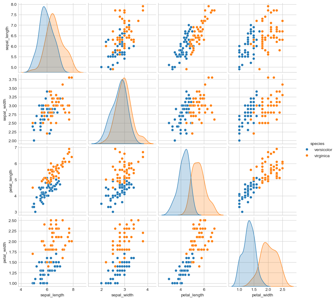
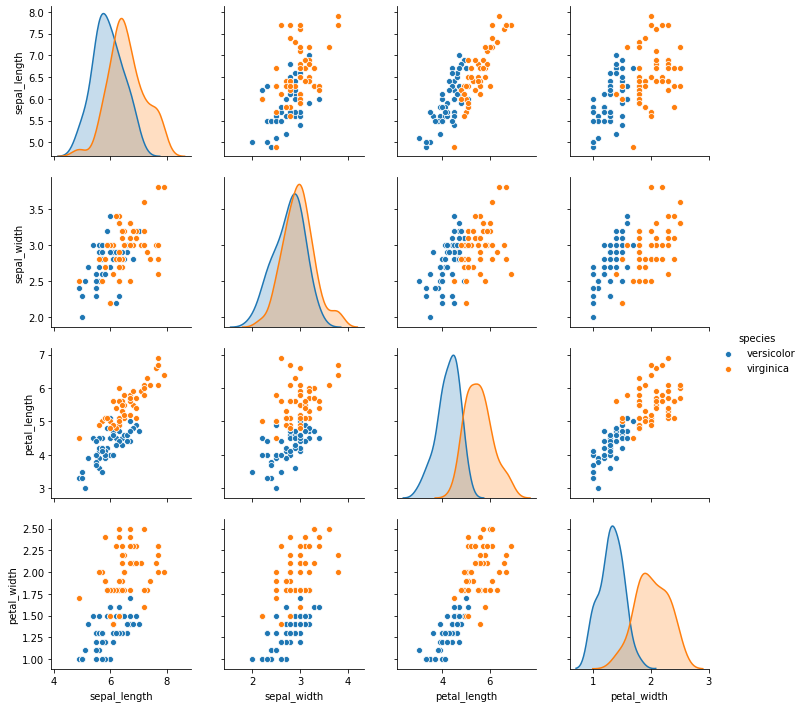
iris = sns.load_dataset("iris")
#g = sns.pairplot(iris, hue="species")
df = iris[iris.species != "setosa"]
g = sns.pairplot(df, hue="species")
df['species_n'] = iris.species.map({'versicolor':1, 'virginica':2})

# Y = 'petal_length', 'petal_width'; X = 'sepal_length', 'sepal_width')
X_iris = np.asarray(df.loc[:, ['sepal_length', 'sepal_width']], dtype=np.float32)
Y_iris = np.asarray(df.loc[:, ['petal_length', 'petal_width']], dtype=np.float32)
label_iris = np.asarray(df.species_n, dtype=int)

# Scale
from sklearn.preprocessing import StandardScaler
scalerx, scalery = StandardScaler(), StandardScaler()
X_iris = scalerx.fit_transform(X_iris)
Y_iris = StandardScaler().fit_transform(Y_iris)

# Split train test
X_iris_tr, X_iris_val, Y_iris_tr, Y_iris_val, label_iris_tr, label_iris_val = \
    sklearn.model_selection.train_test_split(X_iris, Y_iris, label_iris,
                                             train_size=0.5, stratify=label_iris)
/tmp/ipykernel_181680/2720649438.py:5: SettingWithCopyWarning:
A value is trying to be set on a copy of a slice from a DataFrame.
Try using .loc[row_indexer,col_indexer] = value instead

See the caveats in the documentation: https://pandas.pydata.org/pandas-docs/stable/user_guide/indexing.html#returning-a-view-versus-a-copy
  df['species_n'] = iris.species.map({'versicolor':1, 'virginica':2})
Backpropagation with Numpy
This implementation uses Numpy to manually compute the forward pass, loss, and backward pass.
# X=X_iris_tr; Y=Y_iris_tr; X_val=X_iris_val; Y_val=Y_iris_val
def two_layer_regression_numpy_train(X, Y, X_val, Y_val, lr, nite):
# N is batch size; D_in is input dimension;
# H is hidden dimension; D_out is output dimension.
# N, D_in, H, D_out = 64, 1000, 100, 10
N, D_in, H, D_out = X.shape[0], X.shape[1], 100, Y.shape[1]
W1 = np.random.randn(D_in, H)
W2 = np.random.randn(H, D_out)
losses_tr, losses_val = list(), list()
learning_rate = lr
for t in range(nite):
# Forward pass: compute predicted y
z1 = X.dot(W1)
h1 = np.maximum(z1, 0)
Y_pred = h1.dot(W2)
# Compute and print loss
loss = np.square(Y_pred - Y).sum()
# Backprop to compute gradients of w1 and w2 with respect to loss
grad_y_pred = 2.0 * (Y_pred - Y)
grad_w2 = h1.T.dot(grad_y_pred)
grad_h1 = grad_y_pred.dot(W2.T)
grad_z1 = grad_h1.copy()
grad_z1[z1 < 0] = 0
grad_w1 = X.T.dot(grad_z1)
# Update weights
W1 -= learning_rate * grad_w1
W2 -= learning_rate * grad_w2
# Forward pass for validation set: compute predicted y
z1 = X_val.dot(W1)
h1 = np.maximum(z1, 0)
y_pred_val = h1.dot(W2)
loss_val = np.square(y_pred_val - Y_val).sum()
losses_tr.append(loss)
losses_val.append(loss_val)
if t % 10 == 0:
print(t, loss, loss_val)
return W1, W2, losses_tr, losses_val
W1, W2, losses_tr, losses_val = \
two_layer_regression_numpy_train(X=X_iris_tr, Y=Y_iris_tr,
X_val=X_iris_val, Y_val=Y_iris_val,
lr=1e-4, nite=50)
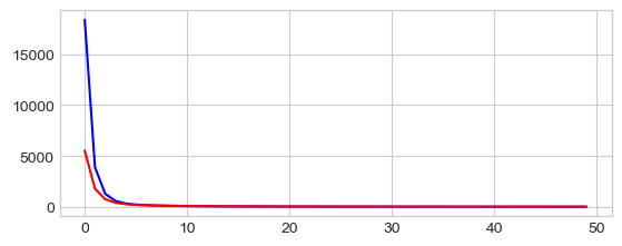
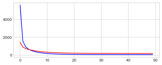
_ = plt.plot(np.arange(len(losses_tr)), losses_tr, "-b",
np.arange(len(losses_val)), losses_val, "-r")
0 8320.86283567932 566.4003298191709
10 69.1144254443256 78.183681464354
20 55.983394365066715 77.33285806985458
30 50.57373709813517 77.19249121024394
40 47.19138471346897 76.77478593928662
Backpropagation with PyTorch Tensors
Learning PyTorch with Examples
Numpy is a great framework, but it cannot utilize GPUs to accelerate its numerical computations. For modern deep neural networks, GPUs often provide speedups of 50x or greater, so unfortunately numpy won’t be enough for modern deep learning. Here we introduce the most fundamental PyTorch concept: the Tensor. A PyTorch Tensor is conceptually identical to a numpy array: a Tensor is an n-dimensional array, and PyTorch provides many functions for operating on these Tensors. Behind the scenes, Tensors can keep track of a computational graph and gradients, but they’re also useful as a generic tool for scientific computing. Also unlike numpy, PyTorch Tensors can utilize GPUs to accelerate their numeric computations. To run a PyTorch Tensor on GPU, you simply need to cast it to a new datatype. Here we use PyTorch Tensors to fit a two-layer network to random data. Like the numpy example above we need to manually implement the forward and backward passes through the network:
import torch

# X=X_iris_tr; Y=Y_iris_tr; X_val=X_iris_val; Y_val=Y_iris_val

def two_layer_regression_tensor_train(X, Y, X_val, Y_val, lr, nite):

    dtype = torch.float
    device = torch.device("cpu")
    # device = torch.device("cuda:0") # Uncomment this to run on GPU

    # N is batch size; D_in is input dimension;
    # H is hidden dimension; D_out is output dimension.
    N, D_in, H, D_out = X.shape[0], X.shape[1], 100, Y.shape[1]

    # Create random input and output data
    X = torch.from_numpy(X)
    Y = torch.from_numpy(Y)
    X_val = torch.from_numpy(X_val)
    Y_val = torch.from_numpy(Y_val)

    # Randomly initialize weights
    W1 = torch.randn(D_in, H, device=device, dtype=dtype)
    W2 = torch.randn(H, D_out, device=device, dtype=dtype)

    losses_tr, losses_val = list(), list()

    learning_rate = lr
    for t in range(nite):
        # Forward pass: compute predicted y
        z1 = X.mm(W1)
        h1 = z1.clamp(min=0)
        y_pred = h1.mm(W2)

        # Compute and print loss
        loss = (y_pred - Y).pow(2).sum().item()

        # Backprop to compute gradients of w1 and w2 with respect to loss
        grad_y_pred = 2.0 * (y_pred - Y)
        grad_w2 = h1.t().mm(grad_y_pred)
        grad_h1 = grad_y_pred.mm(W2.t())
        grad_z1 = grad_h1.clone()
        grad_z1[z1 < 0] = 0
        grad_w1 = X.t().mm(grad_z1)

        # Update weights using gradient descent
        W1 -= learning_rate * grad_w1
        W2 -= learning_rate * grad_w2

        # Forward pass for validation set: compute predicted y
        z1 = X_val.mm(W1)
        h1 = z1.clamp(min=0)
        y_pred_val = h1.mm(W2)
        loss_val = (y_pred_val - Y_val).pow(2).sum().item()

        losses_tr.append(loss)
        losses_val.append(loss_val)

        if t % 10 == 0:
            print(t, loss, loss_val)

    return W1, W2, losses_tr, losses_val

W1, W2, losses_tr, losses_val = \
    two_layer_regression_tensor_train(X=X_iris_tr, Y=Y_iris_tr, X_val=X_iris_val,
                                      Y_val=Y_iris_val,
                                      lr=1e-4, nite=50)

_ = plt.plot(np.arange(len(losses_tr)), losses_tr, "-b",
             np.arange(len(losses_val)), losses_val, "-r")
0 4303.93603515625 418.63006591796875
10 71.38607025146484 116.78504943847656
20 51.27054214477539 87.81427001953125
30 45.72554397583008 80.99897003173828
40 43.343406677246094 78.32192993164062
Backpropagation with PyTorch: Tensors and autograd
Learning PyTorch with Examples
A fully-connected ReLU network with one hidden layer and no biases,
trained to predict y from x by minimizing squared Euclidean distance.
This implementation computes the forward pass using operations on
PyTorch Tensors, and uses PyTorch autograd to compute gradients. A
PyTorch Tensor represents a node in a computational graph. If x is a
Tensor that has x.requires_grad=True then x.grad is another
Tensor holding the gradient of x with respect to some scalar value.
import torch

def two_layer_regression_autograd_train(X, Y, X_val, Y_val, lr, nite):

    dtype = torch.float
    device = torch.device("cpu")
    # device = torch.device("cuda:0") # Uncomment this to run on GPU

    # N is batch size; D_in is input dimension;
    # H is hidden dimension; D_out is output dimension.
    N, D_in, H, D_out = X.shape[0], X.shape[1], 100, Y.shape[1]

    # Setting requires_grad=False indicates that we do not need to compute
    # gradients with respect to these Tensors during the backward pass.
    X = torch.from_numpy(X)
    Y = torch.from_numpy(Y)
    X_val = torch.from_numpy(X_val)
    Y_val = torch.from_numpy(Y_val)

    # Create random Tensors for weights.
    # Setting requires_grad=True indicates that we want to compute gradients
    # with respect to these Tensors during the backward pass.
    W1 = torch.randn(D_in, H, device=device, dtype=dtype, requires_grad=True)
    W2 = torch.randn(H, D_out, device=device, dtype=dtype, requires_grad=True)

    losses_tr, losses_val = list(), list()

    learning_rate = lr
    for t in range(nite):
        # Forward pass: compute predicted y using operations on Tensors; these
        # are exactly the same operations we used to compute the forward pass
        # using Tensors, but we do not need to keep references to intermediate
        # values since we are not implementing the backward pass by hand.
        y_pred = X.mm(W1).clamp(min=0).mm(W2)

        # Compute and print loss using operations on Tensors.
        # Now loss is a Tensor of shape (1,)
        # loss.item() gets the scalar value held in the loss.
        loss = (y_pred - Y).pow(2).sum()

        # Use autograd to compute the backward pass. This call will compute the
        # gradient of loss with respect to all Tensors with requires_grad=True.
        # After this call w1.grad and w2.grad will be Tensors holding the
        # gradient of the loss with respect to w1 and w2 respectively.
        loss.backward()

        # Manually update weights using gradient descent. Wrap in torch.no_grad()
        # because weights have requires_grad=True, but we don't need to track this
        # in autograd.
        # An alternative way is to operate on weight.data and weight.grad.data.
        # Recall that tensor.data gives a tensor that shares the storage with
        # tensor, but doesn't track history.
        # You can also use torch.optim.SGD to achieve this.
        with torch.no_grad():
            W1 -= learning_rate * W1.grad
            W2 -= learning_rate * W2.grad

            # Manually zero the gradients after updating weights
            W1.grad.zero_()
            W2.grad.zero_()

            y_pred = X_val.mm(W1).clamp(min=0).mm(W2)

            # Compute and print loss using operations on Tensors.
            # Now loss is a Tensor of shape (1,)
            # loss.item() gets the scalar value held in the loss.
            loss_val = (y_pred - Y).pow(2).sum()

        if t % 10 == 0:
            print(t, loss.item(), loss_val.item())

        losses_tr.append(loss.item())
        losses_val.append(loss_val.item())

    return W1, W2, losses_tr, losses_val

W1, W2, losses_tr, losses_val = \
    two_layer_regression_autograd_train(X=X_iris_tr, Y=Y_iris_tr,
                                        X_val=X_iris_val, Y_val=Y_iris_val,
                                        lr=1e-4, nite=50)
_ = plt.plot(np.arange(len(losses_tr)), losses_tr, "-b",
             np.arange(len(losses_val)), losses_val, "-r")
0 6619.669921875 4738.6064453125
10 278.9159851074219 521.75732421875
20 93.21061706542969 257.3363037109375
30 64.7365493774414 219.1724853515625
40 56.20269012451172 206.47886657714844
Backpropagation with PyTorch: nn
Learning PyTorch with Examples
This implementation uses the nn package from PyTorch to build the network. PyTorch autograd makes it easy to define computational graphs and take gradients, but raw autograd can be a bit too low-level for defining complex neural networks; this is where the nn package can help. The nn package defines a set of Modules, which you can think of as a neural network layer that has produces output from input and may have some trainable weights.
import torch
def two_layer_regression_nn_train(X, Y, X_val, Y_val, lr, nite):
# N is batch size; D_in is input dimension;
# H is hidden dimension; D_out is output dimension.
N, D_in, H, D_out = X.shape[0], X.shape[1], 100, Y.shape[1]
X = torch.from_numpy(X)
Y = torch.from_numpy(Y)
X_val = torch.from_numpy(X_val)
Y_val = torch.from_numpy(Y_val)
# Use the nn package to define our model as a sequence of layers.
# nn.Sequential is a Module which contains other Modules, and applies
# them in sequence to produce its output. Each Linear Module computes
# output from input using a linear function, and holds internal Tensors
# for its weight and bias.
model = torch.nn.Sequential(
torch.nn.Linear(D_in, H),
torch.nn.ReLU(),
torch.nn.Linear(H, D_out),
)
# The nn package also contains definitions of popular loss functions; in this
# case we will use Mean Squared Error (MSE) as our loss function.
loss_fn = torch.nn.MSELoss(reduction='sum')
losses_tr, losses_val = list(), list()
learning_rate = lr
for t in range(nite):
# Forward pass: compute predicted y by passing x to the model. Module
# objects override the __call__ operator so you can call them like
# functions. When doing so you pass a Tensor of input data to the Module
# and it produces a Tensor of output data.
y_pred = model(X)
# Compute and print loss. We pass Tensors containing the predicted and
# true values of y, and the loss function returns a Tensor containing the
# loss.
loss = loss_fn(y_pred, Y)
# Zero the gradients before running the backward pass.
model.zero_grad()
# Backward pass: compute gradient of the loss with respect to all the
# learnable parameters of the model. Internally, the parameters of each
# Module are stored in Tensors with requires_grad=True, so this call
# will compute gradients for all learnable parameters in the model.
loss.backward()
# Update the weights using gradient descent. Each parameter is a Tensor,
# so we can access its gradients like we did before.
with torch.no_grad():
for param in model.parameters():
param -= learning_rate * param.grad
y_pred = model(X_val)
loss_val = (y_pred - Y_val).pow(2).sum()
if t % 10 == 0:
print(t, loss.item(), loss_val.item())
losses_tr.append(loss.item())
losses_val.append(loss_val.item())
return model, losses_tr, losses_val
model, losses_tr, losses_val = \
two_layer_regression_nn_train(X=X_iris_tr, Y=Y_iris_tr,
X_val=X_iris_val, Y_val=Y_iris_val,
lr=1e-4, nite=50)
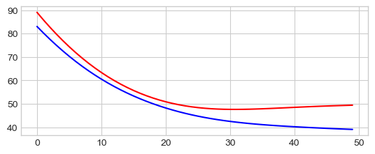
_ = plt.plot(np.arange(len(losses_tr)), losses_tr, "-b",
np.arange(len(losses_val)), losses_val, "-r")
0 60.84171676635742 65.23538970947266
10 42.599857330322266 55.307090759277344
20 38.216976165771484 54.05012130737305
30 36.2943000793457 54.090911865234375
40 35.161956787109375 54.361236572265625
Backpropagation with PyTorch optim
This implementation uses the nn package from PyTorch to build the network. Rather than manually updating the weights of the model as we have been doing, we use the optim package to define an Optimizer that will update the weights for us. The optim package defines many optimization algorithms that are commonly used for deep learning, including SGD+momentum, RMSProp, Adam, etc.
import torch
def two_layer_regression_nn_optim_train(X, Y, X_val, Y_val, lr, nite):
# N is batch size; D_in is input dimension;
# H is hidden dimension; D_out is output dimension.
N, D_in, H, D_out = X.shape[0], X.shape[1], 100, Y.shape[1]
X = torch.from_numpy(X)
Y = torch.from_numpy(Y)
X_val = torch.from_numpy(X_val)
Y_val = torch.from_numpy(Y_val)
# Use the nn package to define our model and loss function.
model = torch.nn.Sequential(
torch.nn.Linear(D_in, H),
torch.nn.ReLU(),
torch.nn.Linear(H, D_out),
)
loss_fn = torch.nn.MSELoss(reduction='sum')
losses_tr, losses_val = list(), list()
# Use the optim package to define an Optimizer that will update the weights of
# the model for us. Here we will use Adam; the optim package contains many
# other optimization algorithm. The first argument to the Adam constructor
# tells the optimizer which Tensors it should update.
learning_rate = lr
optimizer = torch.optim.Adam(model.parameters(), lr=learning_rate)
for t in range(nite):
# Forward pass: compute predicted y by passing x to the model.
y_pred = model(X)
# Compute and print loss.
loss = loss_fn(y_pred, Y)
# Before the backward pass, use the optimizer object to zero all of the
# gradients for the variables it will update (which are the learnable
# weights of the model). This is because by default, gradients are
# accumulated in buffers( i.e, not overwritten) whenever .backward()
# is called. Checkout docs of torch.autograd.backward for more details.
optimizer.zero_grad()
# Backward pass: compute gradient of the loss with respect to model
# parameters
loss.backward()
# Calling the step function on an Optimizer makes an update to its
# parameters
optimizer.step()
with torch.no_grad():
y_pred = model(X_val)
loss_val = loss_fn(y_pred, Y_val)
if t % 10 == 0:
print(t, loss.item(), loss_val.item())
losses_tr.append(loss.item())
losses_val.append(loss_val.item())
return model, losses_tr, losses_val
model, losses_tr, losses_val = \
two_layer_regression_nn_optim_train(X=X_iris_tr, Y=Y_iris_tr,
X_val=X_iris_val, Y_val=Y_iris_val,
lr=1e-3, nite=50)
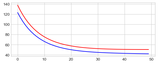
_ = plt.plot(np.arange(len(losses_tr)), losses_tr, "-b",
np.arange(len(losses_val)), losses_val, "-r")
0 121.76207733154297 104.62301635742188
10 81.1495361328125 76.97682189941406
20 56.0490837097168 61.42247772216797
30 43.4493293762207 55.462921142578125
40 38.075889587402344 55.15611267089844