Convolutional Neural Networks (CNNs)
Principles of CNNs
Sources:
CNN Stanford cs231n
Deep learning Stanford cs231n
Pytorch
MNIST and pytorch:
Introduction to CNNs
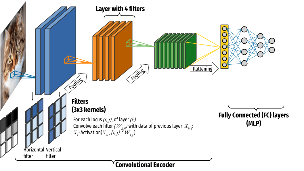
CNNs are deep learning architectures designed for processing grid-like data such as images. Inspired by the biological visual cortex, they learn hierarchical feature representations, making them effective for tasks like image classification, object detection, and segmentation.
Key Principles of CNNs:
Convolutional Layers are the core building block of a CNN, which applies a convolution operation to the input, passing the result to the next layer: it perform feature extraction using learnable filters (kernels), allowing CNNs to detect local patterns such as edges and textures.
Activation Functions introduce non-linearity into the model, enabling the network to learn complex patterns. ReLU (Rectified Linear Unit) is the most commonly used activation function, improving training speed and mitigating vanishing gradients. Possible function are Tanh or Sigmoid and most commonly used the ReLu(Rectified Linear Unit function. ReLu accelerate the training because the derivative of sigmoid becomes very small in the saturating region and therefore the updates to the weights almost vanish. This is called vanishing gradient problem..
Pooling Layers reduces the spatial dimensions (height and width) of the input feature maps by downsampling the input feature maps summarizing the presence of features in patches of the feature map. Max pooling and average pooling are the most common functions.
Fully Connected Layers flatten extracted features and connects to a classifier, typically a softmax layer for classification tasks.
Dropout: reduces the over-fitting by using a Dropout layer after every FC layer. Dropout layer has a probability,(p), associated with it and is applied at every neuron of the response map separately. It randomly switches off the activation with the probability p.
Batch Normalization normalizes the inputs of each layer to have a mean of zero and a variance of one, which improve network stability. This normalization is performed for each mini-batch during training.
CNN Architectures: Evolution from LeNet to ResNet
LeNet-5 (1998)
First successful CNN for handwritten digit recognition.
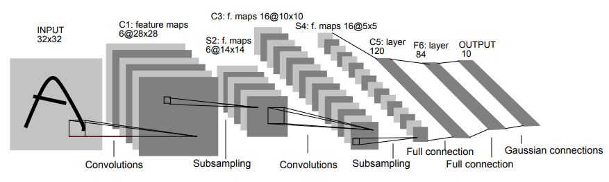
LeNet
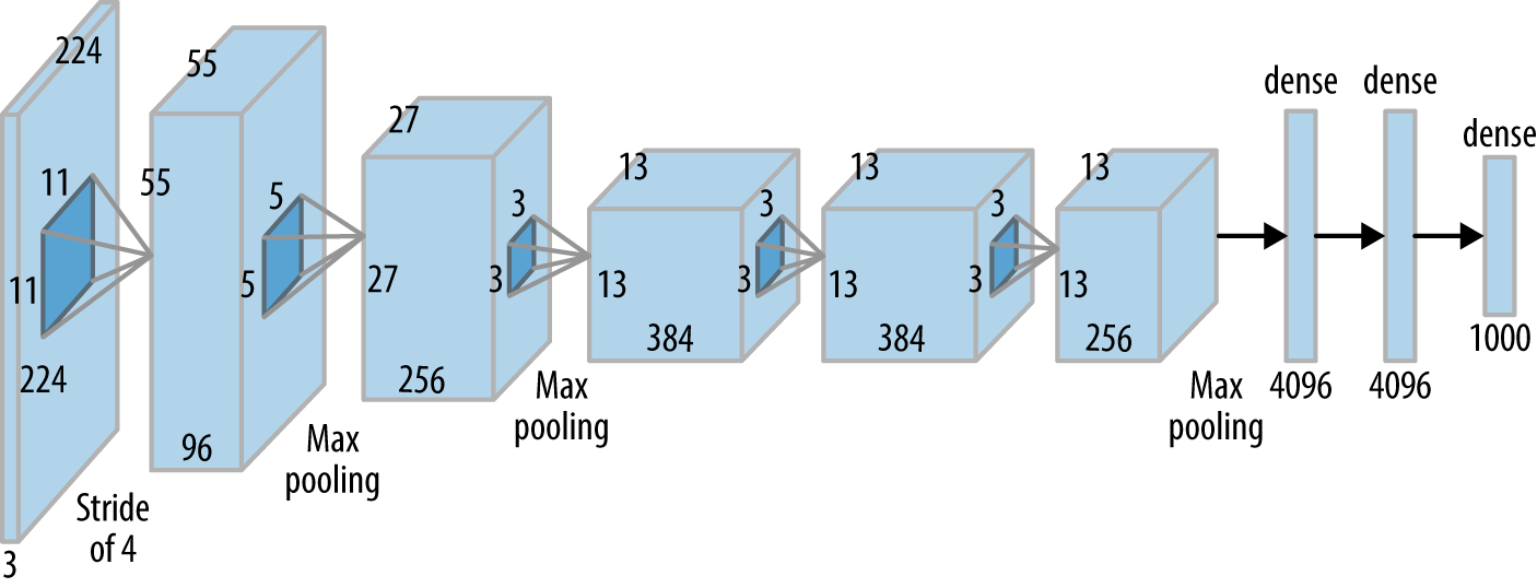
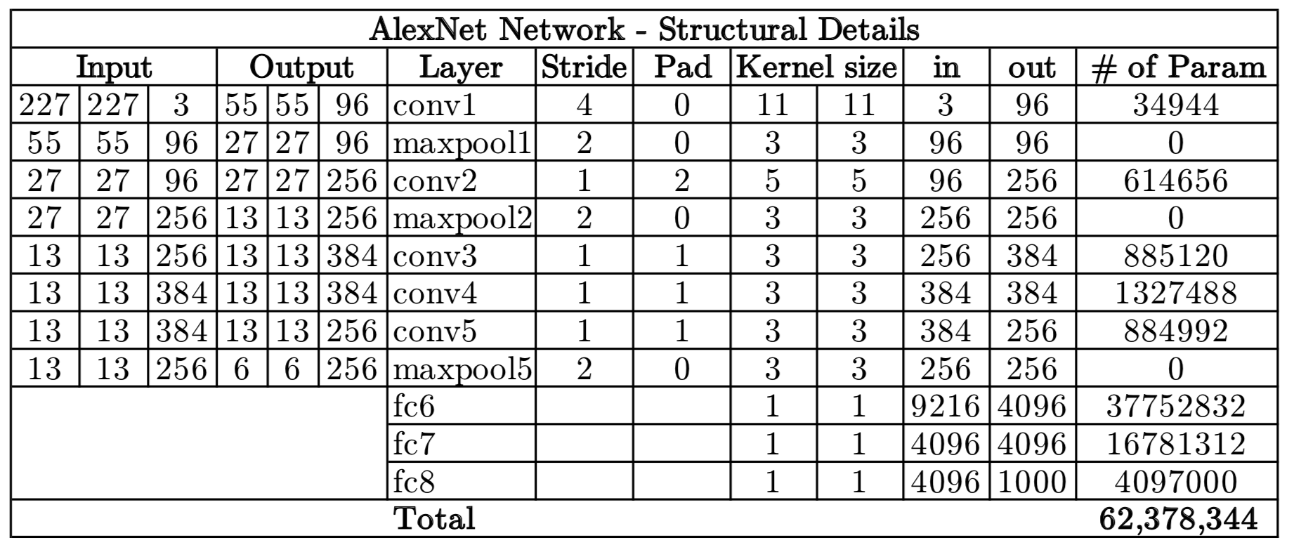
AlexNet (2012)
Revolutionized deep learning by winning the ImageNet competition. Introduced ReLU activation, dropout, and GPU acceleration. Featured Convolutional Layers stacked on top of each other (previously it was common to only have a single CONV layer always immediately followed by a POOL layer).
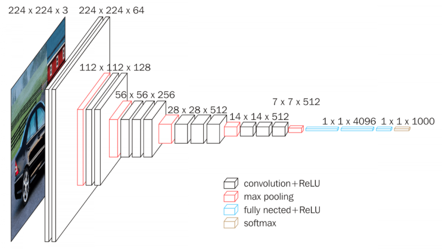
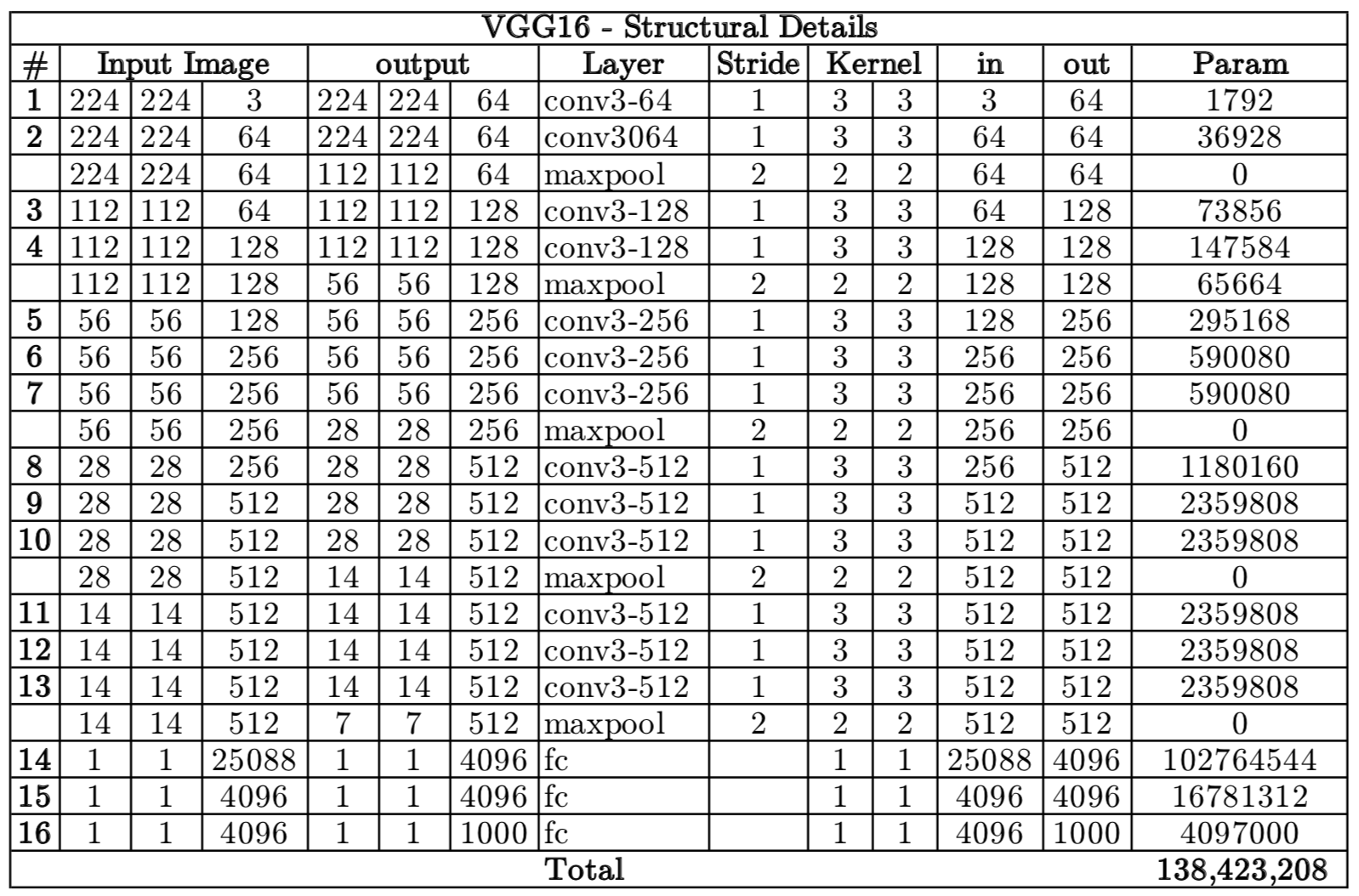
VGG (2014)
Introduced a simple yet deep architecture with 3×3 convolutions.
GoogLeNet (Inception) (2014)
Introduced the Inception module, using multiple kernel sizes in parallel.
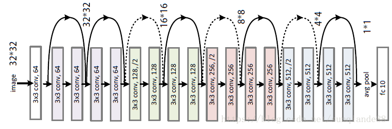
ResNet (2015)
Introduced skip connections, allowing training of very deep networks.
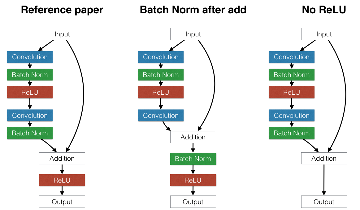
ResNet block
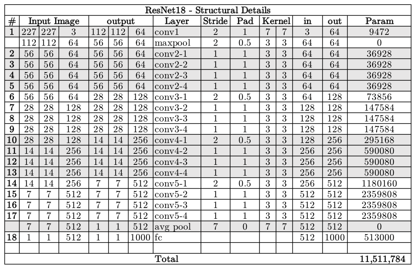
Architectures general guidelines
ConvNets stack CONV,POOL,FC layers
Trend towards smaller filters and deeper architectures: stack 3x3, instead of 5x5
Trend towards getting rid of POOL/FC layers (just CONV)
Historically architectures looked like [(CONV-RELU) x N POOL?] x M (FC-RELU) x K, SOFTMAX where N is usually up to ~5, M is large, 0 <= K <= 2.
But recent advances such as ResNet/GoogLeNet have challenged this paradigm
Conclusion and Further Topics
Recent architectures: EfficientNet, Vision Transformers (ViTs), MobileNet for edge devices.
Advanced topics: Transfer learning, object detection (YOLO, Faster R-CNN), segmentation (U-Net).
Hands-on implementation: Implement CNNs using TensorFlow/PyTorch for real-world applications.
Training function
%matplotlib inline

import os
import numpy as np
from pathlib import Path

# ML
import torch
import torch.nn as nn
import torch.optim as optim
from torch.optim import lr_scheduler
import torchvision
import torchvision.transforms as transforms
from torchvision import models
# Device configuration
device = torch.device('cuda' if torch.cuda.is_available() else 'cpu')
# device = 'cpu' # Force CPU
# print(device)

# Plot
import matplotlib.pyplot as plt
import seaborn as sns

# Plot parameters
plt.style.use('seaborn-v0_8-whitegrid')
fig_w, fig_h = plt.rcParams.get('figure.figsize')
plt.rcParams['figure.figsize'] = (fig_w, fig_h * .5)
%matplotlib inline
See train_val_model function.
from pystatsml.dl_utils import train_val_model
CNN in PyTorch
LeNet-5
Here we implement LeNet-5 with relu activation. Sources:
import torch.nn as nn
import torch.nn.functional as F

class LeNet5(nn.Module):
    """
    layers: (nb channels in input layer,
             nb channels in 1rst conv,
             nb channels in 2nd conv,
             nb neurons for 1rst FC: TO BE TUNED,
             nb neurons for 2nd FC,
             nb neurons for 3rd FC,
             nb neurons output FC TO BE TUNED)
    """
    def __init__(self, layers = (1, 6, 16, 1024, 120, 84, 10), debug=False):
        super(LeNet5, self).__init__()
        self.layers = layers
        self.debug = debug
        self.conv1 = nn.Conv2d(layers[0], layers[1], 5, padding=2)
        self.conv2 = nn.Conv2d(layers[1], layers[2], 5)
        self.fc1   = nn.Linear(layers[3], layers[4])
        self.fc2   = nn.Linear(layers[4], layers[5])
        self.fc3   = nn.Linear(layers[5], layers[6])

    def forward(self, x):
        x = F.max_pool2d(F.relu(self.conv1(x)), 2) # same shape / 2
        x = F.max_pool2d(F.relu(self.conv2(x)), 2) # -4 / 2
        if self.debug:
            print("### DEBUG: Shape of last convnet=",
                  x.shape[1:], ". FC size=", np.prod(x.shape[1:]))
        x = x.view(-1, self.layers[3])
        x = F.relu(self.fc1(x))
        x = F.relu(self.fc2(x))
        x = self.fc3(x)
        return F.log_softmax(x, dim=1)
VGGNet like: conv-relu blocks
# Defining the network (LeNet-5)
import torch.nn as nn
import torch.nn.functional as F

class MiniVGGNet(torch.nn.Module):

    def __init__(self, layers=(1, 16, 32, 1024, 120, 84, 10), debug=False):
        super(MiniVGGNet, self).__init__()
        self.layers = layers
        self.debug = debug

        # Conv block 1
        self.conv11 = nn.Conv2d(in_channels=layers[0],out_channels=layers[1],
                                kernel_size=3, stride=1, padding=0, bias=True)
        self.conv12 = nn.Conv2d(in_channels=layers[1], out_channels=layers[1],
                                kernel_size=3, stride=1, padding=0, bias=True)

        # Conv block 2
        self.conv21 = nn.Conv2d(in_channels=layers[1], out_channels=layers[2],
                                kernel_size=3, stride=1, padding=0, bias=True)
        self.conv22 = nn.Conv2d(in_channels=layers[2], out_channels=layers[2],
                                kernel_size=3, stride=1, padding=1, bias=True)

        # Fully connected layer
        self.fc1   = nn.Linear(layers[3], layers[4])
        self.fc2   = nn.Linear(layers[4], layers[5])
        self.fc3   = nn.Linear(layers[5], layers[6])

    def forward(self, x):
        x = F.relu(self.conv11(x))
        x = F.relu(self.conv12(x))
        x = F.max_pool2d(x, 2)

        x = F.relu(self.conv21(x))
        x = F.relu(self.conv22(x))
        x = F.max_pool2d(x, 2)

        if self.debug:
            print("### DEBUG: Shape of last convnet=", x.shape[1:],
                  ". FC size=", np.prod(x.shape[1:]))
        x = x.view(-1, self.layers[3])
        x = F.relu(self.fc1(x))
        x = F.relu(self.fc2(x))
        x = self.fc3(x)

        return F.log_softmax(x, dim=1)
ResNet-like Model
Stack multiple resnet blocks
# ---------------------------------------------------------------------------- #
# An implementation of https://arxiv.org/pdf/1512.03385.pdf                    #
# See section 4.2 for the model architecture on CIFAR-10                       #
# Some part of the code was referenced from below                              #
# https://github.com/pytorch/vision/blob/master/torchvision/models/resnet.py   #
# ---------------------------------------------------------------------------- #
import torch.nn as nn

# 3x3 convolution
def conv3x3(in_channels, out_channels, stride=1):
    return nn.Conv2d(in_channels, out_channels, kernel_size=3,
                     stride=stride, padding=1, bias=False)

# Residual block
class ResidualBlock(nn.Module):
    def __init__(self, in_channels, out_channels, stride=1, downsample=None):
        super(ResidualBlock, self).__init__()
        self.conv1 = conv3x3(in_channels, out_channels, stride)
        self.bn1 = nn.BatchNorm2d(out_channels)
        self.relu = nn.ReLU(inplace=True)
        self.conv2 = conv3x3(out_channels, out_channels)
        self.bn2 = nn.BatchNorm2d(out_channels)
        self.downsample = downsample

    def forward(self, x):
        residual = x
        out = self.conv1(x)
        out = self.bn1(out)
        out = self.relu(out)
        out = self.conv2(out)
        out = self.bn2(out)
        if self.downsample:
            residual = self.downsample(x)
        out += residual
        out = self.relu(out)
        return out

# ResNet
class ResNet(nn.Module):
    def __init__(self, block, layers, num_classes=10):
        super(ResNet, self).__init__()
        self.in_channels = 16
        self.conv = conv3x3(3, 16)
        self.bn = nn.BatchNorm2d(16)
        self.relu = nn.ReLU(inplace=True)
        self.layer1 = self.make_layer(block, 16, layers[0])
        self.layer2 = self.make_layer(block, 32, layers[1], 2)
        self.layer3 = self.make_layer(block, 64, layers[2], 2)
        self.avg_pool = nn.AvgPool2d(8)
        self.fc = nn.Linear(64, num_classes)

    def make_layer(self, block, out_channels, blocks, stride=1):
        downsample = None
        if (stride != 1) or (self.in_channels != out_channels):
            downsample = nn.Sequential(
                conv3x3(self.in_channels, out_channels, stride=stride),
                nn.BatchNorm2d(out_channels))
        layers = []
        layers.append(block(self.in_channels, out_channels, stride, downsample))
        self.in_channels = out_channels
        for i in range(1, blocks):
            layers.append(block(out_channels, out_channels))
        return nn.Sequential(*layers)

    def forward(self, x):
        out = self.conv(x)
        out = self.bn(out)
        out = self.relu(out)
        out = self.layer1(out)
        out = self.layer2(out)
        out = self.layer3(out)
        out = self.avg_pool(out)
        out = out.view(out.size(0), -1)
        out = self.fc(out)
        return F.log_softmax(out, dim=1)
        #return out
ResNet9
Sources:
Classification: MNIST digits
from pystatsml.datasets import load_mnist_pytorch

dataloaders, WD = load_mnist_pytorch(
    batch_size_train=64, batch_size_test=10000)
os.makedirs(os.path.join(WD, "models"), exist_ok=True)

# Info about the dataset
D_in = np.prod(dataloaders["train"].dataset.data.shape[1:])
D_out = len(dataloaders["train"].dataset.targets.unique())
print("Datasets shapes:", {
      x: dataloaders[x].dataset.data.shape for x in ['train', 'test']})
print("N input features:", D_in, "Output classes:", D_out)
/home/ed203246/data/pystatml/dl_mnist_pytorch
---------------------------------------------------------------------------

NameError                                 Traceback (most recent call last)

Cell In[12], line 8
      5 os.makedirs(os.path.join(WD, "models"), exist_ok=True)
      7 # Info about the dataset
----> 8 D_in = np.prod(dataloaders["train"].dataset.data.shape[1:])
      9 D_out = len(dataloaders["train"].dataset.targets.unique())
     10 print("Datasets shapes:", {
     11       x: dataloaders[x].dataset.data.shape for x in ['train', 'test']})


NameError: name 'np' is not defined
LeNet
Dry run in debug mode to get the shape of the last convnet layer.
model = LeNet5((1, 6, 16, 1, 120, 84, 10), debug=True)
batch_idx, (data_example, target_example) = next(
    enumerate(dataloaders["train"]))
print(model)
_ = model(data_example)
LeNet5(
  (conv1): Conv2d(1, 6, kernel_size=(5, 5), stride=(1, 1), padding=(2, 2))
  (conv2): Conv2d(6, 16, kernel_size=(5, 5), stride=(1, 1))
  (fc1): Linear(in_features=1, out_features=120, bias=True)
  (fc2): Linear(in_features=120, out_features=84, bias=True)
  (fc3): Linear(in_features=84, out_features=10, bias=True)
)
### DEBUG: Shape of last convnet= torch.Size([16, 5, 5]) . FC size= 400
Set First FC layer to 400
model = LeNet5((1, 6, 16, 400, 120, 84, 10)).to(device)
optimizer = optim.SGD(model.parameters(), lr=0.01, momentum=0.5)
criterion = nn.NLLLoss()
# Explore the model
for parameter in model.parameters():
print(parameter.shape)
print("Total number of parameters =", np.sum([np.prod(parameter.shape) for
parameter in model.parameters()]))
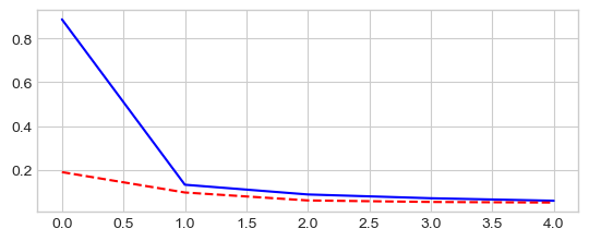
model, losses, accuracies = train_val_model(model, criterion, optimizer,
dataloaders,
num_epochs=5, log_interval=2)
_ = plt.plot(losses['train'], '-b', losses['val'], '--r')
torch.Size([6, 1, 5, 5])
torch.Size([6])
torch.Size([16, 6, 5, 5])
torch.Size([16])
torch.Size([120, 400])
torch.Size([120])
torch.Size([84, 120])
torch.Size([84])
torch.Size([10, 84])
torch.Size([10])
Total number of parameters = 61706
Epoch 0/4
----------
train Loss: 0.8882 Acc: 72.55%
val Loss: 0.1889 Acc: 94.00%

Epoch 2/4
----------
train Loss: 0.0865 Acc: 97.30%
val Loss: 0.0592 Acc: 98.07%

Epoch 4/4
----------
train Loss: 0.0578 Acc: 98.22%
val Loss: 0.0496 Acc: 98.45%

Training complete in 0m 55s
Best val Acc: 98.45%
MiniVGGNet
model = MiniVGGNet(layers=(1, 16, 32, 1, 120, 84, 10), debug=True)

print(model)
_ = model(data_example)
MiniVGGNet(
  (conv11): Conv2d(1, 16, kernel_size=(3, 3), stride=(1, 1))
  (conv12): Conv2d(16, 16, kernel_size=(3, 3), stride=(1, 1))
  (conv21): Conv2d(16, 32, kernel_size=(3, 3), stride=(1, 1))
  (conv22): Conv2d(32, 32, kernel_size=(3, 3), stride=(1, 1), padding=(1, 1))
  (fc1): Linear(in_features=1, out_features=120, bias=True)
  (fc2): Linear(in_features=120, out_features=84, bias=True)
  (fc3): Linear(in_features=84, out_features=10, bias=True)
)
### DEBUG: Shape of last convnet= torch.Size([32, 5, 5]) . FC size= 800
Set First FC layer to 800
model = MiniVGGNet((1, 16, 32, 800, 120, 84, 10)).to(device)
optimizer = optim.SGD(model.parameters(), lr=0.01, momentum=0.5)
criterion = nn.NLLLoss()
# Explore the model
for parameter in model.parameters():
print(parameter.shape)
print("Total number of parameters =",
np.sum([np.prod(parameter.shape)
for parameter in model.parameters()]))
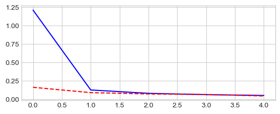
model, losses, accuracies = train_val_model(model, criterion, optimizer,
dataloaders,
num_epochs=5, log_interval=2)
_ = plt.plot(losses['train'], '-b', losses['val'], '--r')
torch.Size([16, 1, 3, 3])
torch.Size([16])
torch.Size([16, 16, 3, 3])
torch.Size([16])
torch.Size([32, 16, 3, 3])
torch.Size([32])
torch.Size([32, 32, 3, 3])
torch.Size([32])
torch.Size([120, 800])
torch.Size([120])
torch.Size([84, 120])
torch.Size([84])
torch.Size([10, 84])
torch.Size([10])
Total number of parameters = 123502
Epoch 0/4
----------
train Loss: 1.2111 Acc: 58.85%
val Loss: 0.1599 Acc: 94.67%

Epoch 2/4
----------
train Loss: 0.0781 Acc: 97.58%
val Loss: 0.0696 Acc: 97.75%

Epoch 4/4
----------
train Loss: 0.0493 Acc: 98.48%
val Loss: 0.0420 Acc: 98.62%

Training complete in 2m 9s
Best val Acc: 98.62%
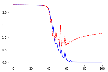
Reduce the size of training dataset
Reduce the size of the training dataset by considering only 10
minibatche for size16.
train_loader, val_loader = dataloaders["train"], dataloaders["test"]

train_size = 10 * 16

# Stratified sub-sampling
targets = train_loader.dataset.targets.numpy()
nclasses = len(set(targets))

indices = np.concatenate([np.random.choice(np.where(targets == lab)[0],
                                           int(train_size / nclasses),
                                           replace=False)
                          for lab in set(targets)])
np.random.shuffle(indices)

train_loader = torch.utils.data.DataLoader(train_loader.dataset, batch_size=16,
                        sampler=torch.utils.data.SubsetRandomSampler(indices))

# Check train subsampling
train_labels = np.concatenate([labels.numpy()
                              for inputs, labels in train_loader])
print("Train size=", len(train_labels), " Train label count=",
      {lab: np.sum(train_labels == lab) for lab in set(train_labels)})
print("Batch sizes=", [inputs.size(0) for inputs, labels in train_loader])

# Put together train and val
dataloaders = dict(train=train_loader, val=val_loader)

# Info about the dataset
data_shape = dataloaders["train"].dataset.data.shape[1:]
D_in = np.prod(data_shape)
D_out = len(dataloaders["train"].dataset.targets.unique())
print("Datasets shape", {x: dataloaders[x].dataset.data.shape
                         for x in ['train', 'val']})
print("N input features", D_in, "N output", D_out)
Train size= 160  Train label count= {np.int64(0): np.int64(16), np.int64(1): np.int64(16), np.int64(2): np.int64(16), np.int64(3): np.int64(16), np.int64(4): np.int64(16), np.int64(5): np.int64(16), np.int64(6): np.int64(16), np.int64(7): np.int64(16), np.int64(8): np.int64(16), np.int64(9): np.int64(16)}
Batch sizes= [16, 16, 16, 16, 16, 16, 16, 16, 16, 16]
Datasets shape {'train': torch.Size([60000, 28, 28]), 'val': torch.Size([10000, 28, 28])}
N input features 784 N output 10
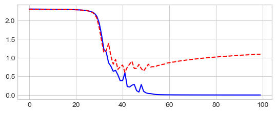
LeNet5
model = LeNet5((1, 6, 16, 400, 120, 84, D_out)).to(device)
optimizer = optim.SGD(model.parameters(), lr=0.01, momentum=0.5)
criterion = nn.NLLLoss()

model, losses, accuracies = train_val_model(model, criterion, optimizer,
                                            dataloaders,
                                            num_epochs=100, log_interval=20)

_ = plt.plot(losses['train'], '-b', losses['val'], '--r')
Epoch 0/99
----------
train Loss: 2.3072 Acc: 7.50%
val Loss: 2.3001 Acc: 8.89%

Epoch 20/99
----------
train Loss: 0.4810 Acc: 83.75%
val Loss: 0.7552 Acc: 72.66%

Epoch 40/99
----------
train Loss: 0.1285 Acc: 95.62%
val Loss: 0.6663 Acc: 81.72%

Epoch 60/99
----------
train Loss: 0.0065 Acc: 100.00%
val Loss: 0.6982 Acc: 84.26%

Epoch 80/99
----------
train Loss: 0.0032 Acc: 100.00%
val Loss: 0.7571 Acc: 84.26%

Training complete in 1m 37s
Best val Acc: 84.34%
MiniVGGNet
model = MiniVGGNet((1, 16, 32, 800, 120, 84, 10)).to(device)
optimizer = optim.SGD(model.parameters(), lr=0.01, momentum=0.5)
criterion = nn.NLLLoss()

model, losses, accuracies = train_val_model(model, criterion, optimizer,
                                            dataloaders,
                                            num_epochs=100, log_interval=20)

_ = plt.plot(losses['train'], '-b', losses['val'], '--r')
Epoch 0/99
----------
train Loss: 2.3048 Acc: 10.00%
val Loss: 2.3026 Acc: 10.28%

Epoch 20/99
----------
train Loss: 2.2865 Acc: 26.25%
val Loss: 2.2861 Acc: 23.22%

Epoch 40/99
----------
train Loss: 0.3847 Acc: 85.00%
val Loss: 0.8042 Acc: 75.76%

Epoch 60/99
----------
train Loss: 0.0047 Acc: 100.00%
val Loss: 0.8659 Acc: 83.57%

Epoch 80/99
----------
train Loss: 0.0013 Acc: 100.00%
val Loss: 1.0183 Acc: 83.39%

Training complete in 4m 39s
Best val Acc: 84.01%
Classification: CIFAR-10 dataset with 10 classes
The CIFAR-10 dataset consists of 60000 32x32 colour images in 10 classes, with 6000 images per class.
Source Yunjey Choi Github pytorch tutorial
Load CIFAR-10 dataset CIFAR-10 Loader
from pystatsml.datasets import load_cifar10_pytorch

dataloaders, _ = load_cifar10_pytorch(
    batch_size_train=100, batch_size_test=100)

# Info about the dataset
D_in = np.prod(dataloaders["train"].dataset.data.shape[1:])
D_out = len(set(dataloaders["train"].dataset.targets))
print("Datasets shape:", {
      x: dataloaders[x].dataset.data.shape for x in dataloaders.keys()})
print("N input features:", D_in, "N output:", D_out)
LeNet
model = LeNet5((3, 6, 16, 1, 120, 84, D_out), debug=True)
batch_idx, (data_example, target_example) = next(enumerate(train_loader))
print(model)
_ = model(data_example)
LeNet5(
  (conv1): Conv2d(3, 6, kernel_size=(5, 5), stride=(1, 1), padding=(2, 2))
  (conv2): Conv2d(6, 16, kernel_size=(5, 5), stride=(1, 1))
  (fc1): Linear(in_features=1, out_features=120, bias=True)
  (fc2): Linear(in_features=120, out_features=84, bias=True)
  (fc3): Linear(in_features=84, out_features=10, bias=True)
)
### DEBUG: Shape of last convnet= torch.Size([16, 6, 6]) . FC size= 576
Set 576 neurons to the first FC layer
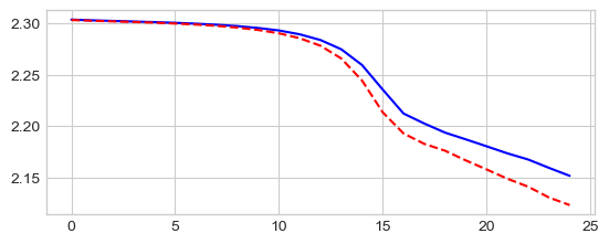
SGD with momentum lr=0.001, momentum=0.5
model = LeNet5((3, 6, 16, 576, 120, 84, D_out)).to(device)
optimizer = optim.SGD(model.parameters(), lr=0.001, momentum=0.5)
criterion = nn.NLLLoss()

# Explore the model
for parameter in model.parameters():
    print(parameter.shape)

print("Total number of parameters =",
      np.sum([np.prod(parameter.shape)
              for parameter in model.parameters()]))

model, losses, accuracies = train_val_model(model, criterion, optimizer,
                                            dataloaders,
                                            num_epochs=25, log_interval=5)

_ = plt.plot(losses['train'], '-b', losses['val'], '--r')
torch.Size([6, 3, 5, 5])
torch.Size([6])
torch.Size([16, 6, 5, 5])
torch.Size([16])
torch.Size([120, 576])
torch.Size([120])
torch.Size([84, 120])
torch.Size([84])
torch.Size([10, 84])
torch.Size([10])
Total number of parameters = 83126
Epoch 0/24
----------
train Loss: 2.3037 Acc: 10.06%
val Loss: 2.3032 Acc: 10.05%

Epoch 5/24
----------
train Loss: 2.3005 Acc: 10.72%
val Loss: 2.2998 Acc: 10.61%

Epoch 10/24
----------
train Loss: 2.2931 Acc: 11.90%
val Loss: 2.2903 Acc: 11.27%

Epoch 15/24
----------
train Loss: 2.2355 Acc: 16.46%
val Loss: 2.2134 Acc: 17.75%

Epoch 20/24
----------
train Loss: 2.1804 Acc: 19.07%
val Loss: 2.1579 Acc: 20.26%

Training complete in 5m 13s
Best val Acc: 23.19%
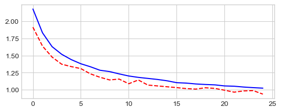
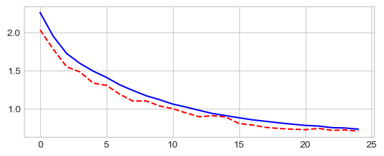
Increase learning rate and momentum lr=0.01, momentum=0.9
model = LeNet5((3, 6, 16, 576, 120, 84, D_out)).to(device)
optimizer = optim.SGD(model.parameters(), lr=0.01, momentum=0.9)
criterion = nn.NLLLoss()

model, losses, accuracies = train_val_model(model, criterion, optimizer,
                                            dataloaders,
                                            num_epochs=25, log_interval=5)

_ = plt.plot(losses['train'], '-b', losses['val'], '--r')
Epoch 0/24
----------
train Loss: 2.1798 Acc: 17.53%
val Loss: 1.9141 Acc: 31.27%

Epoch 5/24
----------
train Loss: 1.3804 Acc: 49.93%
val Loss: 1.3098 Acc: 53.23%

Epoch 10/24
----------
train Loss: 1.2019 Acc: 56.79%
val Loss: 1.0886 Acc: 60.91%

Epoch 15/24
----------
train Loss: 1.1043 Acc: 60.61%
val Loss: 1.0321 Acc: 63.26%

Epoch 20/24
----------
train Loss: 1.0569 Acc: 62.31%
val Loss: 0.9942 Acc: 65.55%

Training complete in 5m 15s
Best val Acc: 67.18%
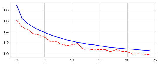
Adaptative learning rate: Adam
model = LeNet5((3, 6, 16, 576, 120, 84, D_out)).to(device)
optimizer = torch.optim.Adam(model.parameters(), lr=0.001)
criterion = nn.NLLLoss()

model, losses, accuracies = train_val_model(model, criterion, optimizer,
                                            dataloaders,
                                            num_epochs=25, log_interval=5)

_ = plt.plot(losses['train'], '-b', losses['val'], '--r')
Epoch 0/24
----------
train Loss: 1.8866 Acc: 29.71%
val Loss: 1.6111 Acc: 40.21%

Epoch 5/24
----------
train Loss: 1.3877 Acc: 49.62%
val Loss: 1.3016 Acc: 53.23%

Epoch 10/24
----------
train Loss: 1.2274 Acc: 55.93%
val Loss: 1.1575 Acc: 58.78%

Epoch 15/24
----------
train Loss: 1.1399 Acc: 59.28%
val Loss: 1.0712 Acc: 61.84%

Epoch 20/24
----------
train Loss: 1.0806 Acc: 61.62%
val Loss: 1.0334 Acc: 62.69%

Training complete in 5m 25s
Best val Acc: 65.14%
MiniVGGNet
model = MiniVGGNet(layers=(3, 16, 32, 1, 120, 84, D_out), debug=True)
print(model)
_ = model(data_example)
MiniVGGNet(
  (conv11): Conv2d(3, 16, kernel_size=(3, 3), stride=(1, 1))
  (conv12): Conv2d(16, 16, kernel_size=(3, 3), stride=(1, 1))
  (conv21): Conv2d(16, 32, kernel_size=(3, 3), stride=(1, 1))
  (conv22): Conv2d(32, 32, kernel_size=(3, 3), stride=(1, 1), padding=(1, 1))
  (fc1): Linear(in_features=1, out_features=120, bias=True)
  (fc2): Linear(in_features=120, out_features=84, bias=True)
  (fc3): Linear(in_features=84, out_features=10, bias=True)
)
### DEBUG: Shape of last convnet= torch.Size([32, 6, 6]) . FC size= 1152
Set 1152 neurons to the first FC layer
SGD with large momentum and learning rate
model = MiniVGGNet((3, 16, 32, 1152, 120, 84, D_out)).to(device)
optimizer = optim.SGD(model.parameters(), lr=0.01, momentum=0.9)
criterion = nn.NLLLoss()

model, losses, accuracies = train_val_model(model, criterion, optimizer,
                                            dataloaders,
                                            num_epochs=25, log_interval=5)

_ = plt.plot(losses['train'], '-b', losses['val'], '--r')
Epoch 0/24
----------
train Loss: 2.2581 Acc: 13.96%
val Loss: 2.0322 Acc: 25.49%

Epoch 5/24
----------
train Loss: 1.4107 Acc: 48.84%
val Loss: 1.3065 Acc: 52.92%

Epoch 10/24
----------
train Loss: 1.0621 Acc: 62.12%
val Loss: 1.0013 Acc: 64.64%

Epoch 15/24
----------
train Loss: 0.8828 Acc: 68.70%
val Loss: 0.8078 Acc: 72.08%

Epoch 20/24
----------
train Loss: 0.7830 Acc: 72.52%
val Loss: 0.7273 Acc: 74.83%

Training complete in 11m 44s
Best val Acc: 75.50%
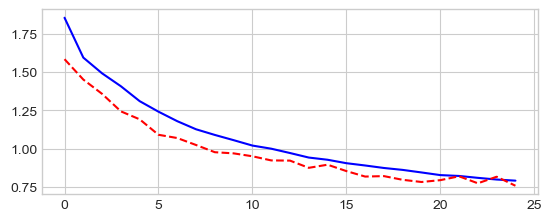
Adam
model = MiniVGGNet((3, 16, 32, 1152, 120, 84, D_out)).to(device)
optimizer = torch.optim.Adam(model.parameters(), lr=0.001)
criterion = nn.NLLLoss()

model, losses, accuracies = \
    train_val_model(model, criterion, optimizer, dataloaders,
                    num_epochs=25, log_interval=5)

_ = plt.plot(losses['train'], '-b', losses['val'], '--r')
Epoch 0/24
----------
train Loss: 1.8556 Acc: 30.40%
val Loss: 1.5847 Acc: 40.66%

Epoch 5/24
----------
train Loss: 1.2417 Acc: 55.39%
val Loss: 1.0908 Acc: 61.45%

Epoch 10/24
----------
train Loss: 1.0203 Acc: 63.66%
val Loss: 0.9503 Acc: 66.19%

Epoch 15/24
----------
train Loss: 0.9051 Acc: 67.98%
val Loss: 0.8536 Acc: 70.10%

Epoch 20/24
----------
train Loss: 0.8273 Acc: 70.74%
val Loss: 0.7942 Acc: 72.55%

Training complete in 11m 60s
Best val Acc: 74.00%
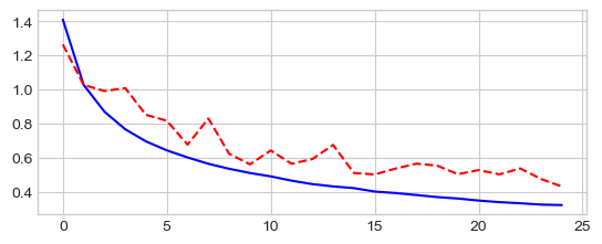
ResNet
model = ResNet(ResidualBlock, [2, 2, 2], num_classes=D_out).to(device)
# 195738 parameters
optimizer = torch.optim.Adam(model.parameters(), lr=0.001)
criterion = nn.NLLLoss()

model, losses, accuracies = \
    train_val_model(model, criterion, optimizer, dataloaders,
                    num_epochs=25, log_interval=5)

_ = plt.plot(losses['train'], '-b', losses['val'], '--r')
Epoch 0/24
----------
train Loss: 1.4107 Acc: 48.21%
val Loss: 1.2645 Acc: 54.80%

Epoch 5/24
----------
train Loss: 0.6440 Acc: 77.60%
val Loss: 0.8178 Acc: 72.40%

Epoch 10/24
----------
train Loss: 0.4914 Acc: 82.89%
val Loss: 0.6432 Acc: 78.16%

Epoch 15/24
----------
train Loss: 0.4024 Acc: 86.27%
val Loss: 0.5026 Acc: 83.43%

Epoch 20/24
----------
train Loss: 0.3496 Acc: 87.86%
val Loss: 0.5282 Acc: 82.18%

Training complete in 58m 9s
Best val Acc: 85.61%
Segmentation with U-Net
Source Segmentation Models:
U-Net is a fully convolutional neural network architecture designed for semantic image segmentation. It consists of two main parts:
An encoder (downsampling path) that extracts increasingly abstract features
A decoder (upsampling path) that gradually recovers spatial details
The key is the use of skip connections between corresponding encoder and decoder layers. These connections allow the decoder to access fine-grained details from earlier encoder layers, which helps produce more precise segmentation masks.
The skip connections work by concatenating feature maps from the encoder directly into the decoder at corresponding resolutions. This helps preserve important spatial information that would otherwise be lost during the encoding process.
Example: Image Segmentation with U-Net using PyTorch
Below is an example of how to implement image segmentation using the U-Net architecture with PyTorch on a real dataset. We will use the Oxford-IIIT Pet Dataset for this example.
Step1: Load the Dataset
We will use the Oxford-IIIT Pet Dataset, which can be downloaded from here. For simplicity, we will assume the dataset is already downloaded and structured as follows:
Step 2: Define the U-Net Model
Here is the implementation of the U-Net model in PyTorch:
import torch
import torch.nn as nn


class UNet(nn.Module):
    def __init__(self, in_channels, out_channels):
        super(UNet, self).__init__()

        def conv_block(in_channels, out_channels):
            return nn.Sequential(
                nn.Conv2d(in_channels, out_channels, kernel_size=3, padding=1),
                nn.ReLU(inplace=True),
                nn.Conv2d(out_channels, out_channels,
                          kernel_size=3, padding=1),
                nn.ReLU(inplace=True)
            )

        def up_conv(in_channels, out_channels):
            return nn.ConvTranspose2d(in_channels, out_channels, kernel_size=2,
                                      stride=2)

        self.enc1 = conv_block(in_channels, 64)
        self.enc2 = conv_block(64, 128)
        self.enc3 = conv_block(128, 256)
        self.enc4 = conv_block(256, 512)

        self.pool = nn.MaxPool2d(kernel_size=2, stride=2)

        self.bottleneck = conv_block(512, 1024)

        self.upconv4 = up_conv(1024, 512)
        self.dec4 = conv_block(1024, 512)
        self.upconv3 = up_conv(512, 256)
        self.dec3 = conv_block(512, 256)
        self.upconv2 = up_conv(256, 128)
        self.dec2 = conv_block(256, 128)
        self.upconv1 = up_conv(128, 64)
        self.dec1 = conv_block(128, 64)

        self.conv_final = nn.Conv2d(64, out_channels, kernel_size=1)

    def forward(self, x):
        enc1 = self.enc1(x)
        enc2 = self.enc2(self.pool(enc1))
        enc3 = self.enc3(self.pool(enc2))
        enc4 = self.enc4(self.pool(enc3))

        bottleneck = self.bottleneck(self.pool(enc4))

        dec4 = self.upconv4(bottleneck)
        dec4 = torch.cat((dec4, enc4), dim=1)
        dec4 = self.dec4(dec4)
        dec3 = self.upconv3(dec4)
        dec3 = torch.cat((dec3, enc3), dim=1)
        dec3 = self.dec3(dec3)
        dec2 = self.upconv2(dec3)
        dec2 = torch.cat((dec2, enc2), dim=1)
        dec2 = self.dec2(dec2)
        dec1 = self.upconv1(dec2)
        dec1 = torch.cat((dec1, enc1), dim=1)
        dec1 = self.dec1(dec1)

        return self.conv_final(dec1)
Step 3: Load and Preprocess the Dataset
We use the torchvision library to load and preprocess the dataset:
from torchvision import transforms
from torch.utils.data import DataLoader, Dataset
from PIL import Image
import os
import os.path
from pathlib import Path

# Directory
DIR = os.path.join(Path.home(), "data", "pystatml", "dl_Oxford-IIITPet")
# <Directory>/images: input images
# <Directory>/annotations: corresponding masks


class PetDataset(Dataset):
    def __init__(self, image_dir, mask_dir, transform=None):
        self.image_dir = image_dir
        self.mask_dir = mask_dir
        self.transform = transform
        self.image_filenames = os.listdir(image_dir)

    def __len__(self):
        return len(self.image_filenames)

    def __getitem__(self, idx):
        img_path = os.path.join(self.image_dir, self.image_filenames[idx])
        mask_path = os.path.join(self.mask_dir,
                            self.image_filenames[idx].replace('.jpg', '.png'))
        image = Image.open(img_path).convert('RGB')
        mask = Image.open(mask_path).convert('L')

        if self.transform:
            image = self.transform(image)
            mask = self.transform(mask)

        return image, mask


transform = transforms.Compose([
    transforms.Resize((128, 128)),
    transforms.ToTensor()
])

dataset = PetDataset(os.path.join(DIR, 'images'),
                     os.path.join(DIR, 'annotations'), transform=transform)
dataloader = DataLoader(dataset, batch_size=4, shuffle=True)
Step 4: Train the U-Net Model
Finally, we will train the U-Net model:
import torch.optim as optim

model = UNet(in_channels=3, out_channels=1)
criterion = nn.BCEWithLogitsLoss()
optimizer = optim.Adam(model.parameters(), lr=0.001)

def train(model, dataloader, criterion, optimizer, num_epochs=1):
    model.train()
    for epoch in range(num_epochs):
        for images, masks in dataloader:
            optimizer.zero_grad()
            outputs = model(images)
            loss = criterion(outputs, masks)
            loss.backward()
            optimizer.step()
        print(f'Epoch [{epoch+1}/{num_epochs}], Loss: {loss.item():.4f}')

# Do not executer (takes 2H)
# train(model, dataloader, criterion, optimizer)
Epoch [1/10], Loss: 0.0414
Epoch [2/10], Loss: 0.0438
Epoch [3/10], Loss: 0.0430
Epoch [4/10], Loss: 0.0402
Epoch [5/10], Loss: 0.0449
Epoch [6/10], Loss: 0.0430
Epoch [7/10], Loss: 0.0438
Epoch [8/10], Loss: 0.0433
Epoch [9/10], Loss: 0.0440
Epoch [10/10], Loss: 0.0453
Save the model and reload the model
model_dirname = os.path.join(DIR, "models")
model_filename = os.path.join(model_dirname, "unet.pt")
os.makedirs(model_dirname, exist_ok=True)

torch.save(model.state_dict(), model_filename)
model_ = UNet(in_channels=3, out_channels=1)
model_.load_state_dict(torch.load(model_filename, weights_only=True))
_ = model_.eval()
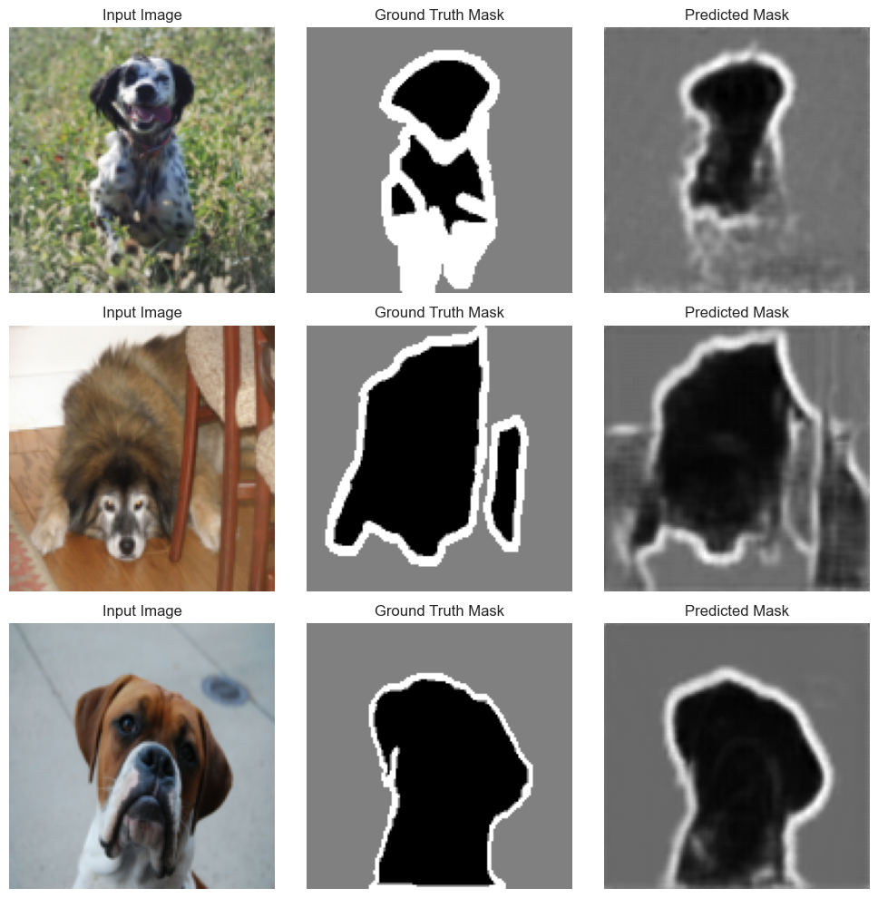
Visualize the results
# Visualize the results
def visualize_results(model, dataloader, num_images=3):
    model.eval()
    images, masks = next(iter(dataloader))
    with torch.no_grad():
        outputs = model(images)
        outputs = torch.sigmoid(outputs)
        outputs = outputs.cpu().numpy()

    images = images.cpu().numpy()
    masks = masks.cpu().numpy()

    fig, axes = plt.subplots(num_images, 3, figsize=(10, 10))
    for i in range(num_images):
        axes[i, 0].imshow(np.transpose(images[i], (1, 2, 0)))
        axes[i, 0].set_title('Input Image')
        axes[i, 0].axis('off')

        axes[i, 1].imshow(masks[i].squeeze(), cmap='gray')
        axes[i, 1].set_title('Ground Truth Mask')
        axes[i, 1].axis('off')

        axes[i, 2].imshow(outputs[i].squeeze(), cmap='gray')
        axes[i, 2].set_title('Predicted Mask')
        axes[i, 2].axis('off')

    plt.tight_layout()
    plt.show()

visualize_results(model, dataloader)
U-Net: Training Image Segmentation Models in PyTorch
A simple pytorch implementation of U-net
PyTorch - Lung Segmentation using pretrained U-net
UNet architecture with pre-trained ResNet34 from segmentation_models.pytorch library which has many inbuilt segmentation architectures with different backbones.
Identify “Pneumothorax” or a collapsed lung from chest x-rays.
Data Augmentation
Train-val Dataset and DataLoader
User defined Loss