Multilayer Perceptron (MLP)
Sources:
Sources:
import os
import numpy as np
import torch
import torch.nn as nn
import torch.nn.functional as F
import torch.optim as optim
from torch.optim import lr_scheduler
# import torchvision
# from torchvision import transforms
# from torchvision import datasets
# from torchvision import models
#
from pathlib import Path
# Plot
import matplotlib.pyplot as plt
import seaborn as sns

# Plot parameters
plt.style.use('seaborn-v0_8-whitegrid')
fig_w, fig_h = plt.rcParams.get('figure.figsize')
plt.rcParams['figure.figsize'] = (fig_w, fig_h * .5)

# Device configuration
device = torch.device('cuda:0' if torch.cuda.is_available() else 'cpu')
# device = 'cpu' # Force CPU
print(device)
cpu
Single Layer Softmax Classifier (Multinomial Logistic Regression)
Recall of Binary logistic regression
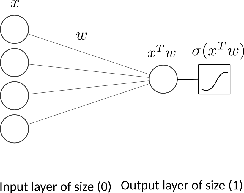
One neuron as output layer
Where
Input: \(\boldsymbol{x}\): a vector of dimension \((p)\) (layer 0).
Parameters: \(\boldsymbol{w}\): a vector of dimension \((p)\) (layer 1). \(b\) is the scalar bias.
Output: \(f(\boldsymbol{x})\) a vector of dimension 1.
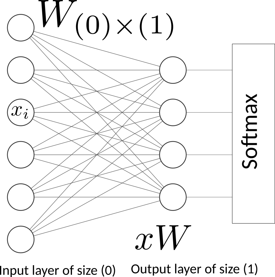
With multinomial logistic regression we have \(k\) possible labels to predict. If we consider the MNIST Handwritten Digit Recognition, the inputs is a \(28 \times 28=784\) image and the output is a vector of \(k=10\) labels or probabilities.
Multinomial Logistic Regression on MINST
Input: \(\boldsymbol{x}\): a vector of dimension \((p=784)\) (layer 0).
Parameters: \(\boldsymbol{W}\): the matrix of coefficients of dimension \((p \times k)\) (layer 1). \(b\) is a \((k)\)-dimentional vector of bias.
Output: \(f(\boldsymbol{x})\) a vector of dimension \((k=10)\) possible labels
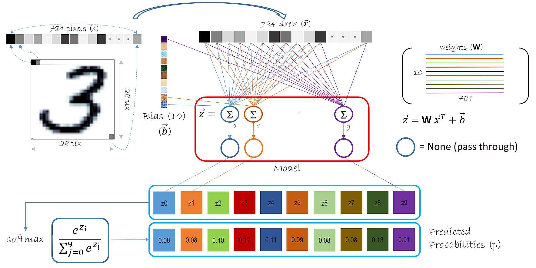
The softmax function is a crucial component in many machine learning and deep learning models, particularly in the context of classification tasks. It is used to convert a vector of raw scores (logits) into a probability distribution. Here’s a detailed explanation of the softmax function: The softmax function takes a vector of real numbers as input and outputs a vector of probabilities that sum to 1. The formula for the softmax function is:
where: - \(z_i\) is the \(i\)-th element of the input vector \(\mathbf{z}\). - \(e\) is the base of the natural logarithm. - The sum in the denominator is over all elements of the input vector.
Softmax Properties
Probability Distribution: The output of the softmax function is a probability distribution, meaning that all the outputs are non-negative and sum to 1.
Exponential Function: The use of the exponential function ensures that the outputs are positive and that larger input values correspond to larger probabilities.
Normalization: The softmax function normalizes the input values by dividing by the sum of the exponentials of all input values, ensuring that the outputs sum to 1
MNIST classfification using multinomial logistic
source: Logistic regression MNIST
Here we fit a multinomial logistic regression with L2 penalty on a subset of the MNIST digits classification task.
Hyperparameters
Dataset: MNIST Handwritten Digit Recognition
from pystatsml.datasets import load_mnist_pytorch

dataloaders, WD = load_mnist_pytorch(
    batch_size_train=64, batch_size_test=10000)
os.makedirs(os.path.join(WD, "models"), exist_ok=True)

# Info about the dataset
D_in = np.prod(dataloaders["train"].dataset.data.shape[1:])
D_out = len(dataloaders["train"].dataset.targets.unique())
print("Datasets shapes:", {
      x: dataloaders[x].dataset.data.shape for x in ['train', 'test']})
print("N input features:", D_in, "Output classes:", D_out)
/home/ed203246/data/pystatml/dl_mnist_pytorch
Datasets shapes: {'train': torch.Size([60000, 28, 28]), 'test': torch.Size([10000, 28, 28])}
N input features: 784 Output classes: 10
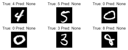
Now let’s take a look at some mini-batches examples.
batch_idx, (example_data, example_targets) = next(
    enumerate(dataloaders["train"]))
print("Train batch:", example_data.shape, example_targets.shape)
batch_idx, (example_data, example_targets) = next(
    enumerate(dataloaders["test"]))
print("Val batch:", example_data.shape, example_targets.shape)
Train batch: torch.Size([64, 1, 28, 28]) torch.Size([64])
Val batch: torch.Size([10000, 1, 28, 28]) torch.Size([10000])
So one test data batch is a tensor of shape: . This means we have 1000 examples of 28x28 pixels in grayscale (i.e. no rgb channels, hence the one). We can plot some of them using matplotlib.
def show_data_label_prediction(data, y_true, y_pred=None, shape=(2, 3)):
    y_pred = [None] * len(y_true) if y_pred is None else y_pred
    fig = plt.figure()
    for i in range(np.prod(shape)):
        plt.subplot(*shape, i+1)
        plt.tight_layout()
        plt.imshow(data[i][0], cmap='gray', interpolation='none')
        plt.title("True: {} Pred: {}".format(y_true[i], y_pred[i]))
        plt.xticks([])
        plt.yticks([])


show_data_label_prediction(
    data=example_data, y_true=example_targets, y_pred=None, shape=(2, 3))
X_train = dataloaders["train"].dataset.data.numpy()
X_train = X_train.reshape((X_train.shape[0], -1))
y_train = dataloaders["train"].dataset.targets.numpy()

X_test = dataloaders["test"].dataset.data.numpy()
X_test = X_test.reshape((X_test.shape[0], -1))
y_test = dataloaders["test"].dataset.targets.numpy()

print(X_train.shape, y_train.shape)
(60000, 784) (60000,)
import matplotlib.pyplot as plt
import numpy as np

from sklearn.linear_model import LogisticRegression
# from sklearn.model_selection import train_test_split
from sklearn.preprocessing import StandardScaler
from sklearn.utils import check_random_state

scaler = StandardScaler()
X_train = scaler.fit_transform(X_train)
X_test = scaler.transform(X_test)

# Turn up tolerance for faster convergence
clf = LogisticRegression(C=50., solver='sag', tol=0.1)
clf.fit(X_train, y_train)
# sparsity = np.mean(clf.coef_ == 0) * 100
score = clf.score(X_test, y_test)

print("Test score with penalty: %.4f" % score)
Test score with penalty: 0.8997
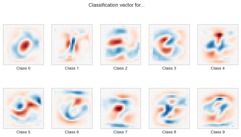
coef = clf.coef_.copy()
plt.figure(figsize=(10, 5))
scale = np.abs(coef).max()
for i in range(10):
    l1_plot = plt.subplot(2, 5, i + 1)
    l1_plot.imshow(coef[i].reshape(28, 28), interpolation='nearest',
                   cmap=plt.cm.RdBu, vmin=-scale, vmax=scale)
    l1_plot.set_xticks(())
    l1_plot.set_yticks(())
    l1_plot.set_xlabel('Class %i' % i)
plt.suptitle('Classification vector for...')

plt.show()
Model: Two Layer MLP
MLP with Scikit-learn
from sklearn.neural_network import MLPClassifier
mlp = MLPClassifier(hidden_layer_sizes=(100, ), max_iter=10, alpha=1e-4,
solver='sgd', verbose=10, tol=1e-4, random_state=1,
learning_rate_init=0.01, batch_size=64)
mlp.fit(X_train, y_train)
print("Training set score: %f" % mlp.score(X_train, y_train))
print("Test set score: %f" % mlp.score(X_test, y_test))
print("Coef shape=", len(mlp.coefs_))
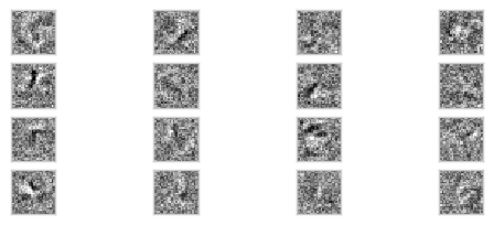
fig, axes = plt.subplots(4, 4)
# use global min / max to ensure all weights are shown on the same scale
vmin, vmax = mlp.coefs_[0].min(), mlp.coefs_[0].max()
for coef, ax in zip(mlp.coefs_[0].T, axes.ravel()):
ax.matshow(coef.reshape(28, 28), cmap=plt.cm.gray, vmin=.5 * vmin,
vmax=.5 * vmax)
ax.set_xticks(())
ax.set_yticks(())
plt.show()
Iteration 1, loss = 0.28828673
Iteration 2, loss = 0.13388073
Iteration 3, loss = 0.09366379
Iteration 4, loss = 0.07317648
Iteration 5, loss = 0.05340251
Iteration 6, loss = 0.04468092
Iteration 7, loss = 0.03548097
Iteration 8, loss = 0.02862098
Iteration 9, loss = 0.02449230
Iteration 10, loss = 0.01874513
/home/ed203246/git/pystatsml/.pixi/envs/default/lib/python3.12/site-packages/sklearn/neural_network/_multilayer_perceptron.py:690: ConvergenceWarning: Stochastic Optimizer: Maximum iterations (10) reached and the optimization hasn't converged yet.
  warnings.warn(
Training set score: 0.997800
Test set score: 0.974900
Coef shape= 2
MLP with pytorch
class TwoLayerMLP(nn.Module):

    def __init__(self, d_in, d_hidden, d_out):
        super(TwoLayerMLP, self).__init__()
        self.d_in = d_in

        self.linear1 = nn.Linear(d_in, d_hidden)
        self.linear2 = nn.Linear(d_hidden, d_out)

    def forward(self, X):
        X = X.view(-1, self.d_in)
        X = self.linear1(X)
        return F.log_softmax(self.linear2(X), dim=1)
Train the Model
First we want to make sure our network is in training mode.
Iterate over epochs
Alternate train and validation dataset
Iterate over all training/val data once per epoch. Loading the individual batches is handled by the DataLoader.
Set the gradients to zero using
optimizer.zero_grad()since PyTorch by default accumulates gradients.Forward pass:
model(inputs): Produce the output of our network.torch.max(outputs, 1): softmax predictions.criterion(outputs, labels): loss between the output and the ground truth label.
In training mode, backward pass
backward(): collect a new set of gradients which we propagate back into each of the network’s parameters usingoptimizer.step().We’ll also keep track of the progress with some printouts. In order to create a nice training curve later on we also create two lists for saving training and testing losses. On the x-axis we want to display the number of training examples the network has seen during training.
Save model state: Neural network modules as well as optimizers have the ability to save and load their internal state using
.state_dict(). With this we can continue training from previously saved state dicts if needed - we’d just need to call.load_state_dict(state_dict).
See train_val_model function.
from pystatsml.dl_utils import train_val_model
Save and reload PyTorch model
PyTorch doc: Save and reload PyTorch model:Note “If you only plan to keep the best performing model (according to the acquired validation loss), don’t forget that best_model_state = model.state_dict() returns a reference to the state and not its copy! You must serialize best_model_state or use best_model_state = deepcopy(model.state_dict()) otherwise your best best_model_state will keep getting updated by the subsequent training iterations. As a result, the final model state will be the state of the overfitted model.”
Save/Load state_dict (Recommended) Save:
import torch
from copy import deepcopy
torch.save(deepcopy(model.state_dict()), PATH)
Load:
model = TheModelClass(*args, **kwargs)
model.load_state_dict(torch.load(PATH, weights_only=True))
model.eval()
Run one epoch and save the model
from copy import deepcopy

model = TwoLayerMLP(D_in, 50, D_out).to(device)
print(next(model.parameters()).is_cuda)
optimizer = optim.SGD(model.parameters(), lr=0.01, momentum=0.5)
criterion = nn.NLLLoss()

# Explore the model
for parameter in model.parameters():
    print(parameter.shape)

print("Total number of parameters =", np.sum(
    [np.prod(parameter.shape) for parameter in model.parameters()]))

model, losses, accuracies = \
    train_val_model(model, criterion, optimizer, dataloaders,
                    num_epochs=1, log_interval=1)

print(next(model.parameters()).is_cuda)
torch.save(deepcopy(model.state_dict()),
           os.path.join(WD, 'models/mod-%s.pth' % model.__class__.__name__))
False
torch.Size([50, 784])
torch.Size([50])
torch.Size([10, 50])
torch.Size([10])
Total number of parameters = 39760
Epoch 0/0
----------
train Loss: 0.4500 Acc: 87.61%
test Loss: 0.3059 Acc: 91.05%

Training complete in 0m 5s
Best val Acc: 91.05%
False
Reload model
model_ = TwoLayerMLP(D_in, 50, D_out)
model_.load_state_dict(torch.load(os.path.join(
    WD, 'models/mod-%s.pth' % model.__class__.__name__), weights_only=True))
model_.to(device)
TwoLayerMLP(
  (linear1): Linear(in_features=784, out_features=50, bias=True)
  (linear2): Linear(in_features=50, out_features=10, bias=True)
)
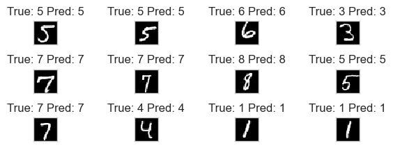
Use the model to make new predictions. Consider the device, ie, load
data on device example_data.to(device) from prediction, then move
back to cpu example_data.cpu().
batch_idx, (example_data, example_targets) = next(
    enumerate(dataloaders["test"]))
example_data = example_data.to(device)

with torch.no_grad():
    output = model(example_data).cpu()

example_data = example_data.cpu()

# Softmax predictions
preds = output.argmax(dim=1)

print("Output shape=", output.shape, "label shape=", preds.shape)
print("Accuracy = {:.2f}%".format(
    (example_targets == preds).sum().item() * 100. / len(example_targets)))

show_data_label_prediction(
    data=example_data, y_true=example_targets, y_pred=preds, shape=(3, 4))
Output shape= torch.Size([10000, 10]) label shape= torch.Size([10000])
Accuracy = 91.05%
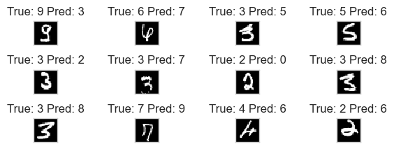
Plot missclassified samples
errors = example_targets != preds
# print(errors, np.where(errors))
print("Nb errors = {}, (Error rate = {:.2f}%)".format(
    errors.sum(), 100 * errors.sum().item() / len(errors)))
err_idx = np.where(errors)[0]
show_data_label_prediction(data=example_data[err_idx],
                           y_true=example_targets[err_idx],
                           y_pred=preds[err_idx], shape=(3, 4))
Nb errors = 895, (Error rate = 8.95%)
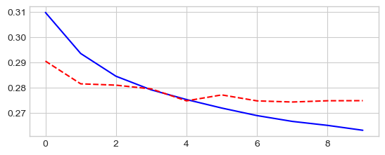
Continue training from checkpoints: reload the model and run 10 more epochs
model = TwoLayerMLP(D_in, 50, D_out)
model.load_state_dict(torch.load(os.path.join(
WD, 'models/mod-%s.pth' % model.__class__.__name__), weights_only=False))
model.to(device)
optimizer = optim.SGD(model.parameters(), lr=0.01, momentum=0.5)
criterion = nn.NLLLoss()
model, losses, accuracies = \
train_val_model(model, criterion, optimizer, dataloaders,
num_epochs=10, log_interval=2)
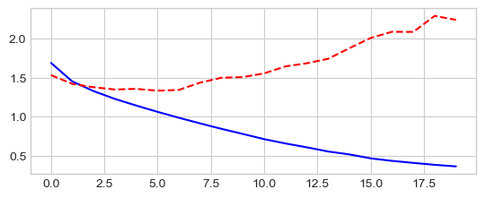
_ = plt.plot(losses['train'], '-b', losses['test'], '--r')
Epoch 0/9
----------
train Loss: 0.3097 Acc: 91.11%
test Loss: 0.2904 Acc: 91.91%

Epoch 2/9
----------
train Loss: 0.2844 Acc: 91.94%
test Loss: 0.2809 Acc: 92.10%

Epoch 4/9
----------
train Loss: 0.2752 Acc: 92.21%
test Loss: 0.2747 Acc: 92.23%

Epoch 6/9
----------
train Loss: 0.2688 Acc: 92.45%
test Loss: 0.2747 Acc: 92.17%

Epoch 8/9
----------
train Loss: 0.2650 Acc: 92.64%
test Loss: 0.2747 Acc: 92.32%

Training complete in 0m 40s
Best val Acc: 92.32%
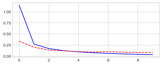
Test several MLP architectures
Define a
MultiLayerMLP([D_in, 512, 256, 128, 64, D_out])class that take the size of the layers as parameters of the constructor.Add some non-linearity with relu acivation function
class MLP(nn.Module):

    def __init__(self, d_layer):
        super(MLP, self).__init__()
        self.d_layer = d_layer
        # Add linear layers
        layer_list = [nn.Linear(d_layer[l], d_layer[l+1])
                      for l in range(len(d_layer) - 1)]
        self.linears = nn.ModuleList(layer_list)

    def forward(self, X):
        X = X.view(-1, self.d_layer[0])
        # relu(Wl x) for all hidden layer
        for layer in self.linears[:-1]:
            X = F.relu(layer(X))
        # softmax(Wl x) for output layer
        return F.log_softmax(self.linears[-1](X), dim=1)
model = MLP([D_in, 512, 256, 128, 64, D_out]).to(device)

optimizer = optim.SGD(model.parameters(), lr=0.01, momentum=0.5)
criterion = nn.NLLLoss()

model, losses, accuracies = \
    train_val_model(model, criterion, optimizer, dataloaders,
                    num_epochs=10, log_interval=2)

_ = plt.plot(losses['train'], '-b', losses['test'], '--r')
Epoch 0/9
----------
train Loss: 1.1449 Acc: 64.01%
test Loss: 0.3366 Acc: 89.96%

Epoch 2/9
----------
train Loss: 0.1693 Acc: 95.00%
test Loss: 0.1361 Acc: 96.11%

Epoch 4/9
----------
train Loss: 0.0946 Acc: 97.21%
test Loss: 0.0992 Acc: 96.94%

Epoch 6/9
----------
train Loss: 0.0606 Acc: 98.20%
test Loss: 0.1002 Acc: 96.97%

Epoch 8/9
----------
train Loss: 0.0395 Acc: 98.87%
test Loss: 0.0833 Acc: 97.42%

Training complete in 1m 11s
Best val Acc: 97.60%
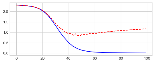
Reduce the size of training dataset
Reduce the size of the training dataset by considering only 10
minibatche for size16.
train_size = 10 * 16

# Stratified sub-sampling
targets = dataloaders["train"].dataset.targets.numpy()
nclasses = len(set(targets))

indices = np.concatenate([np.random.choice(np.where(targets == lab)[0],
                                           int(train_size / nclasses),
                                           replace=False)
                          for lab in set(targets)])
np.random.shuffle(indices)

train_loader = \
    torch.utils.data.DataLoader(dataloaders["train"].dataset,
                        batch_size=16,
                        sampler=torch.utils.data.SubsetRandomSampler(indices))

# Check train subsampling
train_labels = np.concatenate([labels.numpy()
                              for inputs, labels in train_loader])
print("Train size=", len(train_labels), " Train label count=",
      {lab: np.sum(train_labels == lab) for lab in set(train_labels)})
print("Batch sizes=", [inputs.size(0) for inputs, labels in train_loader])

# Put together train and val
dataloaders = dict(train=train_loader, test=dataloaders["test"])

# Info about the dataset
D_in = np.prod(dataloaders["train"].dataset.data.shape[1:])
D_out = len(dataloaders["train"].dataset.targets.unique())
print("Datasets shape", {x: dataloaders[x].dataset.data.shape
                         for x in dataloaders.keys()})
print("N input features", D_in, "N output", D_out)
Train size= 160  Train label count= {np.int64(0): np.int64(16), np.int64(1): np.int64(16), np.int64(2): np.int64(16), np.int64(3): np.int64(16), np.int64(4): np.int64(16), np.int64(5): np.int64(16), np.int64(6): np.int64(16), np.int64(7): np.int64(16), np.int64(8): np.int64(16), np.int64(9): np.int64(16)}
Batch sizes= [16, 16, 16, 16, 16, 16, 16, 16, 16, 16]
Datasets shape {'train': torch.Size([60000, 28, 28]), 'test': torch.Size([10000, 28, 28])}
N input features 784 N output 10
model = MLP([D_in, 512, 256, 128, 64, D_out]).to(device)
optimizer = optim.SGD(model.parameters(), lr=0.01, momentum=0.5)
criterion = nn.NLLLoss()

model, losses, accuracies = \
    train_val_model(model, criterion, optimizer, dataloaders,
                    num_epochs=100, log_interval=20)

_ = plt.plot(losses['train'], '-b', losses['test'], '--r')
Epoch 0/99
----------
train Loss: 2.3042 Acc: 10.00%
test Loss: 2.3013 Acc: 9.80%

Epoch 20/99
----------
train Loss: 2.0282 Acc: 30.63%
test Loss: 2.0468 Acc: 24.58%

Epoch 40/99
----------
train Loss: 0.4945 Acc: 88.75%
test Loss: 0.9630 Acc: 66.42%

Epoch 60/99
----------
train Loss: 0.0483 Acc: 100.00%
test Loss: 0.9570 Acc: 74.40%

Epoch 80/99
----------
train Loss: 0.0145 Acc: 100.00%
test Loss: 1.0840 Acc: 74.40%

Training complete in 1m 7s
Best val Acc: 75.32%
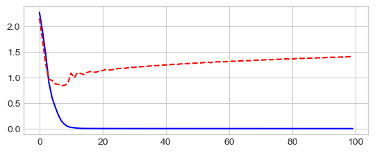
Use an opimizer with an adaptative learning rate: Adam
model = MLP([D_in, 512, 256, 128, 64, D_out]).to(device)
optimizer = torch.optim.Adam(model.parameters(), lr=0.001)
criterion = nn.NLLLoss()

model, losses, accuracies = \
    train_val_model(model, criterion, optimizer, dataloaders,
                    num_epochs=100, log_interval=20)

_ = plt.plot(losses['train'], '-b', losses['test'], '--r')
Epoch 0/99
----------
train Loss: 2.2763 Acc: 15.00%
test Loss: 2.1595 Acc: 45.78%

Epoch 20/99
----------
train Loss: 0.0010 Acc: 100.00%
test Loss: 1.1346 Acc: 77.06%

Epoch 40/99
----------
train Loss: 0.0003 Acc: 100.00%
test Loss: 1.2461 Acc: 76.97%

Epoch 60/99
----------
train Loss: 0.0001 Acc: 100.00%
test Loss: 1.3149 Acc: 77.00%

Epoch 80/99
----------
train Loss: 0.0001 Acc: 100.00%
test Loss: 1.3633 Acc: 77.07%

Training complete in 1m 6s
Best val Acc: 77.54%
Run MLP on CIFAR-10 dataset
The CIFAR-10 dataset consists of 60000 32x32 colour images in 10 classes, with 6000 images per class. There are 50000 training images and 10000 test images.
The dataset is divided into five training batches and one test batch, each with 10000 images. The test batch contains exactly 1000 randomly-selected images from each class. The training batches contain the remaining images in random order, but some training batches may contain more images from one class than another. Between them, the training batches contain exactly 5000 images from each class. The ten classes are: airplane, automobile, bird, cat, deer, dog, frog, horse, ship, truck
Load CIFAR-10 dataset CIFAR-10 Loader
from pystatsml.datasets import load_cifar10_pytorch

dataloaders, _ = load_cifar10_pytorch(
    batch_size_train=100, batch_size_test=100)

# Info about the dataset
D_in = np.prod(dataloaders["train"].dataset.data.shape[1:])
D_out = len(set(dataloaders["train"].dataset.targets))
print("Datasets shape:", {
      x: dataloaders[x].dataset.data.shape for x in dataloaders.keys()})
print("N input features:", D_in, "N output:", D_out)
Files already downloaded and verified
Files already downloaded and verified
Datasets shape: {'train': (50000, 32, 32, 3), 'test': (10000, 32, 32, 3)}
N input features: 3072 N output: 10
Run MLP Classifier with hidden layers of sizes: 512, 256, 128, and 64:
model = MLP([D_in, 512, 256, 128, 64, D_out]).to(device)
optimizer = torch.optim.Adam(model.parameters(), lr=0.001)
criterion = nn.NLLLoss()

model, losses, accuracies = \
    train_val_model(model, criterion, optimizer, dataloaders,
                    num_epochs=20, log_interval=10)

_ = plt.plot(losses['train'], '-b', losses['test'], '--r')
Epoch 0/19
----------
train Loss: 1.6872 Acc: 39.50%
test Loss: 1.5318 Acc: 45.31%

Epoch 10/19
----------
train Loss: 0.7136 Acc: 74.50%
test Loss: 1.5536 Acc: 54.77%

Training complete in 4m 3s
Best val Acc: 54.84%