Numerical Differentiation

import numpy as np

# Plot
import matplotlib.pyplot as plt
import seaborn as sns
#import pystatsml.plot_utils

# Plot parameters
plt.style.use('seaborn-v0_8-whitegrid')
fig_w, fig_h = plt.rcParams.get('figure.figsize')
plt.rcParams['figure.figsize'] = (fig_w, fig_h * .5)
colors = plt.rcParams['axes.prop_cycle'].by_key()['color']
%matplotlib inline

Sources:

• Patrick Walls course of Dept of Mathematics, University of British Columbia.

• Wikipedia

The derivative of a function at is the limit

\[f'(x) = \lim_{h \to 0} \frac{f(x+h) - f(x)}{h}\]

For a fixed step size \(h\), the previous formula provides the slope of the function using the forward difference approximation of the derivative. Equivalently, the slope could be estimated using backward approximation with positions \(x - h\) and \(x\).

The most efficient numerical derivative use the central difference formula with step size is the average of the forward and backward approximation (known as symmetric difference quotient):

\[f'(a) \approx \frac{1}{2} \left( \frac{f(a + h) - f(a)}{h} + \frac{f(a) - f(a - h)}{h} \right) = \frac{f(a + h) - f(a - h)}{2h}\]

Chose the step size depends of two issues

1. Numerical precision: if \(h\) is chosen too small, the subtraction will yield a large rounding error due to cancellation will produce a value of zero. For basic central differences, the optimal (Sauer, Timothy (2012). Numerical Analysis. Pearson. p.248.) step is the cube-root of machine epsilon (\(2.2*10^{-16}\) for double precision), i.e.: \(h\approx 10^{-5}\):

eps = np.finfo(np.float64).eps
print("Machine epsilon: {:e}, Min step size: {:e}".format(eps, np.cbrt(eps)))

Machine epsilon: 2.220446e-16, Min step size: 6.055454e-06

2. The error of the central difference approximation is upper bounded by a function in \(\mathcal{O}(h^2)\). I.e., large step size \(h=10^{-2}\) leads to large error of \(10^{-4}\). Small step size e.g., \(h=10^{-4}\) provide accurate slope estimation in \(10^{-8}\).

Those two points argue for a step size \(h \in [10^{-3}, 10^{-6}]\)

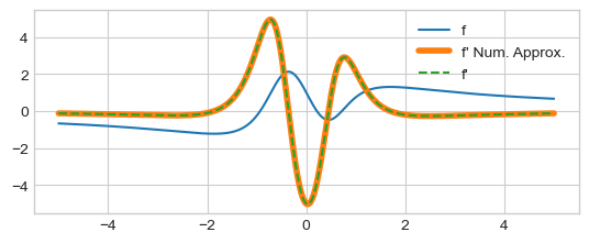
Example: Numerical differentiation of the function:

\[f(x) = \frac{7x^3-5x+1}{2x^4+x^2+1} \ , \ x \in [-5,5]\]

Numerical differentiation with Numpy gradient given values y and x (or spacing dx) of a function.

range_ = [-5, 5]
dx = 1e-3
n = int((range_[1] - range_[0]) / dx)
x = np.linspace(range_[0], range_[1], n)
f = lambda x:  (7 * x ** 3  - 5 * x + 1) / (2 * x ** 4 + x ** 2 + 1)

y = f(x) # values
dydx = np.gradient(y, dx) # values

Symbolic differentiation with sympy to compute true derivative \(f'\)

Installation:

conda install conda-forge::sympy

import sympy as sp
from sympy import lambdify
x_s  = sp.symbols('x', real=True) # defining the variables

f_sym = (7 * x_s ** 3  - 5 * x_s + 1) / (2 * x_s ** 4 + x_s ** 2 + 1)
dfdx_sym =  sp.simplify(sp.diff(f_sym))
print("f =", f_sym)
print("f'=", dfdx_sym)
dfdx_sym = lambdify(x_s, dfdx_sym,  "numpy")

f = (7*x**3 - 5*x + 1)/(2*x**4 + x**2 + 1)
f'= (-14*x**6 + 37*x**4 - 8*x**3 + 26*x**2 - 2*x - 5)/(4*x**8 + 4*x**6 + 5*x**4 + 2*x**2 + 1)

plt.plot(x, y, label="f")
plt.plot(x[1:-1], dydx[1:-1], lw=4, label="f' Num. Approx.")
plt.plot(x, dfdx_sym(x), "--", label="f'")
plt.legend()
plt.show()

Numerical differentiation with numdifftools

The numdifftools numerical differentiation problems in one or more variables.

Installation:

conda install conda-forge::numdifftools

numdifftools.Derivative computes the derivatives of order 1 through 10 on any scalar function. It takes a function f as argument and return a function dfdx that compute the derivatives at x values. Example of first and second order derivative of \(f(x) = x^2, f^\prime(x) = 2 x, f^{\prime\prime}(x) = 2\):

import numdifftools as nd

# Example f(x) = x ** 2

# First order derivative: dfdx = 2 x
print("dfdx = 2 x:", nd.Derivative(lambda x: x ** 2)([1, 2, 3]))

# Second order derivative df^2dx^2 = 2 (Cte)
print("df2dx2 = 2:", nd.Derivative(lambda x: x ** 2, n=2)([1, 2, 3]))

dfdx = 2 x: [2. 4. 6.]
df2dx2 = 2: [2. 2. 2.]

Example with \(f=x^3 - 27 x - 1\). We have \(f^\prime= 3x^2 - 27\), with roots \((-3, 3)\), and \(f^{\prime\prime}=6x\), with root \(0\).

range_ = [-5.5, 5.5]
dx = 1e-3
n = int((range_[1] - range_[0]) / dx)
x = np.linspace(range_[0], range_[1], n)
f = lambda x:  1 * (x ** 3) - 27 * x - 1

# First derivative (! callable function, not values)
dfdx = nd.Derivative(f)

# Second derivative  (! callable function, not values)
df2dx2 = nd.Derivative(f, n=2)

Second-order derivative, “the rate of change of the rate of change” corresponds to the curvature or concavity of the function.

x = np.linspace(range_[0], range_[1], n)
plt.plot(x, f(x), color=colors[0], lw=2, label="f")
plt.plot(x, dfdx(x),  color=colors[1], label="f'")
plt.plot(x, df2dx2(x), color=colors[2], label="f''")
plt.axvline(x=-3, ls='--', color=colors[1])
plt.axvline(x= 3, ls='--', color=colors[1])
plt.axvline(x= 0, ls='--', color=colors[2])
plt.legend()
plt.show()

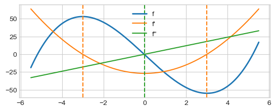
• \(f'' < 0, x<0, f\) is concave down.

• \(f'' > 0, x>0\), \(f\) is concave up.

• \(f'' = 0, x=0\), is an inflection point.

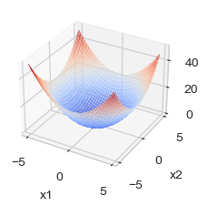
Multivariate functions

\(f(\textbf{x})\) is function of a vector \(\textbf{x}\) of several \(p\) variables \(\textbf{x} = [x_1, ..., x_p]^T\).

Example: \(f(x, y) = x^2 + y^2\)

f = lambda x:  x[0] ** 2 + x[1] ** 2

import matplotlib.pyplot as plt
from matplotlib import cm

# Make data.
x = np.arange(-5, 5, 0.25)
y = np.arange(-5, 5, 0.25)
xx, yy = np.meshgrid(x, y)

zz = f([xx, yy])

# Plot
fig, ax = plt.subplots(subplot_kw={"projection": "3d"})

# Plot the surface.
surf = ax.plot_surface(xx, yy, zz, cmap=cm.coolwarm,
                       linewidth=0, antialiased=False, alpha=0.5, zorder=10)
ax.set_xlabel('x1')
ax.set_ylabel('x2')

Text(0.5, 0.5, 'x2')

The Gradient at a given point \(\textbf{x}\) is the vector of partial derivative of \(f\) at gives the direction of fastest increase.

\[\begin{split}\nabla f(\textbf{x}) = \begin{bmatrix} \partial f / \partial x_1 \\ \vdots \\ \partial f / \partial x_p \end{bmatrix},\end{split}\]

f_grad = nd.Gradient(f)
print(f_grad([0, 0]))
print(f_grad([1, 1]))
print(f_grad([-1, 2]))

[0. 0.]
[2. 2.]
[-2.  4.]

The Hessian matrix contains the second-order partial derivatives of \(f\). It describes the local curvature of a function of many variables. It is noted:

\[\begin{split}f''(\textbf{x}_k) = \nabla^2 f(\textbf{x}_k) = \textbf{H}_{f(\textbf{x}_k)}= \begin{bmatrix} \frac{\partial^2 f}{\partial^2x_1} \ldots \frac{\partial^2 f}{\partial x_p \partial x_1}\\ \vdots \\ \frac{\partial^2 f}{\partial x_1 \partial x_p} \ldots \frac{\partial^2 f}{\partial^2x_p} \end{bmatrix},\end{split}\]

H = nd.Hessian(f)([0, 0])
print(H)

[[2. 0.]
 [0. 2.]]

Numerical Integration

• Principles Patrick Walls course.

• Library: Scipy integrate package.

import numpy as np

# Plot
import matplotlib.pyplot as plt
import seaborn as sns
#import pystatsml.plot_utils

# Plot parameters
plt.style.use('seaborn-v0_8-whitegrid')
fig_w, fig_h = plt.rcParams.get('figure.figsize')
plt.rcParams['figure.figsize'] = (fig_w, fig_h * .5)
%matplotlib inline

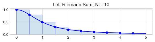
Methods for integrating functions given fixed samples: \([(x_1, f(x_1)), ..., (x_i, f(x_i)), ...(x_N, f(x_N)]\).

Riemann sums of rectangles to approximate the area.

\[\sum_{i=1}^N f(x_i^ * ) (x_i - x_{i-1}) \ \ , \ x_i^* \in [x_{i-1},x_i]\]

The error is in \(\mathcal{O}(\frac{1}{N})\)

f = lambda x : 1 / (1 + x ** 2)
a, b, N = 0, 5, 10
dx = (b - a) / N

x = np.linspace(a, b, N+1)
y = f(x)

x_ = np.linspace(a,b, 10*N+1) # 10 * N points to plot the function smoothly
plt.plot(x_, f(x_), 'b')
x_left = x[:-1] # Left endpoints
y_left = y[:-1]
plt.plot(x_left,y_left,'b.',markersize=10)
plt.bar(x_left,y_left,width=dx, alpha=0.2,align='edge',edgecolor='b')
plt.title('Left Riemann Sum, N = {}'.format(N))

Text(0.5, 1.0, 'Left Riemann Sum, N = 10')

Compute Riemann sums with 100 points

a, b, N = 0, 5, 50
dx = (b - a) / N
x = np.linspace(a, b, N+1)

y = f(x)
print("Integral:", np.sum(f(x[:-1]) * np.diff(x)))

Integral: 1.4214653634808756

Trapezoid Rule sum the trapezoids connecting the points. The error is in \(\mathcal{O}(\frac{1}{N^2})\). Use scipy.integrate.trapezoid function:

from scipy import integrate
integrate.trapezoid(f(x[:-1]), dx=dx)

np.float64(1.369466163161004)

Simpson’s rule uses a quadratic polynomial on each subinterval of a partition to approximate the function and to compute the definite integral. The error is in \(\mathcal{O}(\frac{1}{N^4})\). Use scipy.integrate.simpson function:

from scipy import integrate
integrate.simpson(f(x[:-1]), dx=dx)

np.float64(1.3694791829077122)

Gauss-Legendre Quadrature approximate the integral of a function as a weighted sum of Legendre polynomials.

Methods for Integrating functions given function object \(f()\) that could be evaluated for any value \(x\) in a range \([a, b]\).

Use scipy.integrate.quad function. The first argument to quad is a “callable” Python object (i.e., a function, method, or class instance). Notice the use of a lambda- function in this case as the argument. The next two arguments are the limits of integration.

import scipy.integrate as integrate
integrate.quad(f, a=a, b=b)

(1.3734007669450166, 7.167069904541812e-09)

The return values are the estimated of the integral and the estimate of the absolute integration error.