Optimization (Minimization) by Gradient Descent

Gradient Descent

Optimization (minimization) by gradient descent

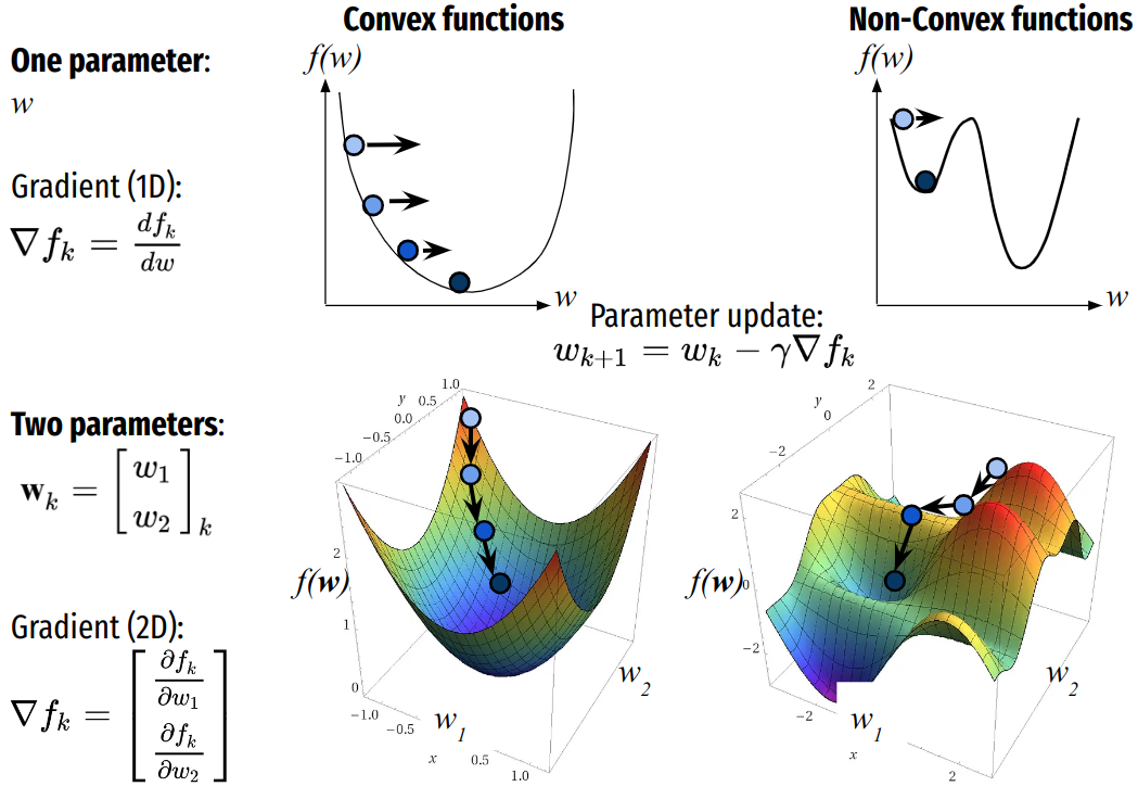
Gradient descent is an optimization algorithm to minimize a cost or loss function \(f\) given its parameter \(w\). The algorithm iteratively moves in the direction of steepest descent as defined by the opposite direction the gradient. In machine learning, we use gradient descent to update the parameters of our model. Parameters refer to coefficients in Linear Regression and weights in neural networks.

Local minimization of \(f\) at point \(x_k\) make use of first-order Taylor expansion local estimation of \(f\) (in one dimension):

\[f(w_k + t) \approx f(w_k) + f'(w_k)t\]

Therefore, to minimize \(f(w_k + t)\) we just have to move in the opposite direction of the derivative \(f'(w_k)\):

\[w_{k+1} = w_{k} - \gamma f'(w_{k})\]

With a learning rate \(\gamma\) that determines the step size at each iteration while moving toward a minimum of a cost function.

In multidimensional problems \(\textbf{w}_{k} \in \mathbb{R}^p\), where:

\[\begin{split}\textbf{w}_k = \begin{bmatrix} w_1 \\ \vdots \\ w_p \end{bmatrix}_k,\end{split}\]

the derivative \(f'(\textbf{w}_k)\) is the gradient (direction) of \(f\) at \(\textbf{w}_k\):

\[\begin{split}\nabla f(\textbf{w}_{k}) = \begin{bmatrix} \partial f / \partial w_1 \\ \vdots \\ \partial f / \partial w_p \end{bmatrix}_k,\end{split}\]

Leading to the minimization scheme:

\[\textbf{w}_{k+1} = \textbf{w}_{k} - \gamma \nabla f(\textbf{w}_{k})\]

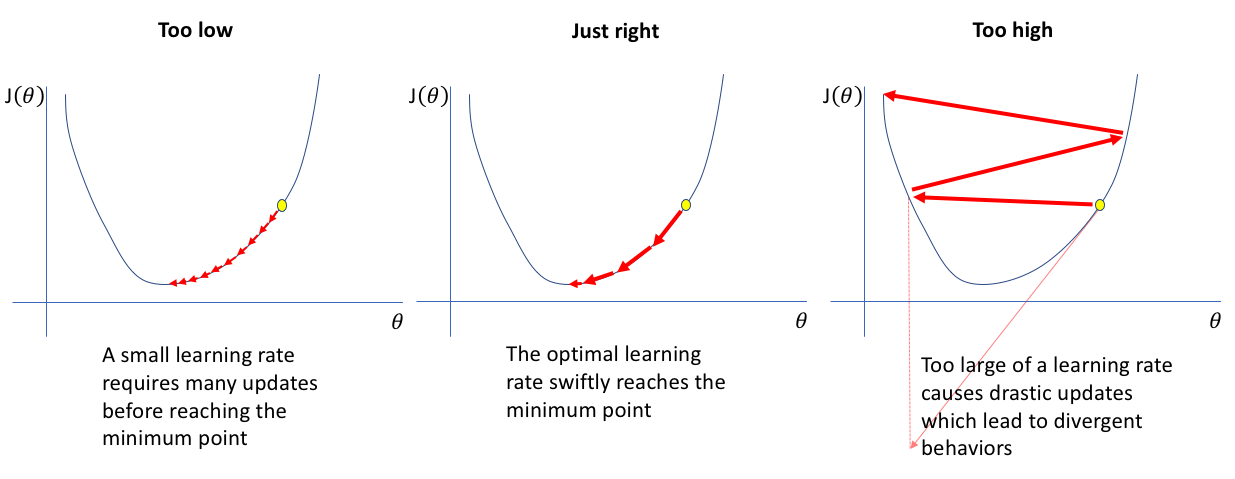
Choosing the Step Size

With large learning rate \(\gamma\) we can cover more ground each step, but we risk overshooting the lowest point since the slope of the hill is constantly changing.

With a very small learning rate**, we can confidently move in the direction of the negative gradient since we are recalculating it so frequently. A small learning rate is more precise, but calculating the gradient is time-consuming, leading too slow convergence

jeremyjordan

Line search can be used (or more sophisticated Backtracking line search) to find value of \(\gamma\) such that \(f(\textbf{w}_{k} - \gamma \nabla f(\textbf{w}_{k}))\) is minimum. However such simple method ignore possible change of the curvature.

• Benefit of gradient decent: simplicity and versatility, almost any function with a gradient can be minimized.

• Limitations:

  • Local minima (local optimization) for non-convex problem.

  • Convergence speed: With fast changing curvature (gradient direction) the estimation of gradient will rapidly become wrong moving away from \(x_k\) suggesting small step-size. This also suggest the integration of change of the gradient direction in the calculus of the step size.

Libraries

import numpy as np
import pandas as pd
from scipy.optimize import minimize
import numdifftools as nd

# Plot
import matplotlib.pyplot as plt
from matplotlib import cm # color map
import seaborn as sns

# Plot parameters
plt.style.use('seaborn-v0_8-whitegrid')
fig_w, fig_h = plt.rcParams.get('figure.figsize')
plt.rcParams['figure.figsize'] = (fig_w, fig_h * 1.)
colors = plt.rcParams['axes.prop_cycle'].by_key()['color']
#%matplotlib inline

Gradient Descent Algorithm

def gradient_descent(fun, x0, args=(), method="first-order", jac=None,
                     hess=None, tol=1.5e-08,
                     options=dict(learning_rate=0.01,
                                  maxiter=1000,
                                  intermediate_res=False)):
    """ Gradient Descent minimization.
    To make API compatible with scipy.optimize.minimize, it takes a
    required fun parameters that is not used and an optional jac
    that is used to compute the gradient.

    Parameters
    ----------
    fun : callable
        The objective function to be minimized.
    x0 : ndarray, shape (n_features,)
        Initial guess.
    args : tuple, optional
        Extra arguments passed to the objective function and its derivatives
        (fun, jac and hess functions)
    method : string, optional
        the solver, by default "first-order" if the basic first-order gradient
        descent.
    jac : callable, optional
        Method for computing the gradient vector, the Jacobian.,
        by default None.
        jac(x, *args) -> array_like, shape (n_features,)
    hess : callable, optional
        Method for computing the Hessian matrix, by default None
        hess(x, *args) -> ndarray, (n_features, n_features)
    tol : float, optional
        Tolerance for termination. Default = 1.5e-08,
        sqrt(np.finfo(np.float64).eps)
    options : dict, optional
        A dictionary of solver options., by default dict(learning_rate=0.01,
        maxiter=1000, intermediate_res=False)

    Returns
    -------
    ndarray, shape (n_features,): the solution, intermediate_res dict

    """
    # Initialize parameters
    weights_k = x0.copy()

    # Termination criteria
    k, eps = 0, np.inf
    # Dict to store intermediate results
    intermediate_res = dict(eps=[], weights=[])

    # Perform gradient descent
    while eps > tol and k < options["maxiter"]:
    #for k in range(options["maxiter"]):
        weights_prev = weights_k.copy()
        weights_grad = jac(weights_k, *args)
        # Update the parameters
        if method == "first-order" and "learning_rate" in options:
            weights_k -= options["learning_rate"] * weights_grad
        if method == "Newton" and hess is not None:
            H = hess(weights_k, *args)
            Hinv = np.linalg.inv(H)
            weights_k -= options["learning_rate"] * np.dot(Hinv, weights_grad)

        # Update termination criteria
        k, eps = k + 1, np.sum((weights_k - weights_prev) ** 2)

        if options["intermediate_res"]:
            intermediate_res["eps"].append(eps)
            intermediate_res["weights"].append(weights_prev)

    return weights_k, intermediate_res

Gradient Descent with Exact Gradient

Minimize:

\[\begin{split}f(\textbf{w}) = f(x, y) = x^2 + y^2 + x y\\ \nabla f(\textbf{w}) = \begin{bmatrix} \partial f / \partial x \\ \partial f / \partial y\end{bmatrix} = \begin{bmatrix} 2 x + 1\\ 2 y + 1\end{bmatrix},\end{split}\]

def f(x):
    x = np.asarray(x)
    x, y = (x[0], x[1]) if x.ndim == 1 else (x[:, 0], x[:, 1])
    return  x ** 2 + y ** 2 + 1 * x * y


print("f:", f([[1, 2],[3, 4]]))
print("f:", f([1, 2]), f([3, 4]))

def f_grad(x):
    x = np.asarray(x, dtype=float)
    x, y = (x[0], x[1]) if x.ndim == 1 else (x[:, 0], x[:, 1])
    return  np.array([2 * x + 1, 2 * y + 1])

print("Grad f:", f_grad([1, 1]))
print("Grad f:", f_grad([1, 2]))
print("Grad f:", f_grad([5, 5]))

f: [ 7 37]
f: 7 37
Grad f: [3. 3.]
Grad f: [3. 5.]
Grad f: [11. 11.]

x0 = np.array([30., 40.])
lr = 0.1
weights_sol, intermediate_res = \
    gradient_descent(fun=f, x0=x0, jac=f_grad,
                     options=dict(learning_rate=lr,
                                  maxiter=100,
                                  intermediate_res=True))

res_ = pd.DataFrame(intermediate_res)
print(res_.head(5))
print(res_.tail(5))
print("Solution: ", weights_sol)

          eps                        weights
0  102.820000                   [30.0, 40.0]
1   65.804800                   [23.9, 31.9]
2   42.115072    [19.02, 25.419999999999998]
3   26.953646   [15.116, 20.235999999999997]
4   17.250333  [11.992799999999999, 16.0888]
             eps                                      weights
47  7.989809e-08   [-0.499149784089306, -0.49887102477432443]
48  5.113478e-08   [-0.4993198272714448, -0.4990968198194595]
49  3.272626e-08  [-0.49945586181715584, -0.4992774558555676]
50  2.094480e-08   [-0.4995646894537247, -0.4994219646844541]
51  1.340467e-08  [-0.49965175156297975, -0.4995375717475633]
Solution:  [-0.4997214  -0.49963006]

Plot solution functions

def plot_surface(x_range, y_range, f, surf=True, wireframe=False):
    x, y = np.linspace(x_range[0], x_range[1], 100), np.linspace(y_range[0], y_range[1], 100)
    #x, y = np.arange(-5, 5, 0.25), np.arange(-5, 5, 0.25)
    xx, yy = np.meshgrid(x, y)
    zz = f(np.column_stack((xx.ravel(), yy.ravel()))).reshape(xx.shape)

    # Figure
    fig, ax = plt.subplots(subplot_kw={"projection": "3d"})

    # Plot the surface.
    if surf:
        surf = ax.plot_surface(xx, yy, zz, cmap=cm.coolwarm,
                        linewidth=0, antialiased=True, alpha=0.5, zorder=10)
    if wireframe:
        ax.plot_wireframe(xx, yy, zz, rstride=2, cstride=2, color='gray', alpha=0.5, lw=1)

    ax.set_xlabel('x'); ax.set_ylabel('y')
    return ax, (xx, yy, zz)

def crop(x, x_range, y_range):
    mask = (x[:, 0] >= x_range[0]) & (x[:, 0] <= x_range[1]) &\
        (x[:, 1] >= y_range[0]) & (x[:, 1] <= y_range[1])
    return x[mask]
    #return x[np.all((x >= min) & (x <= max), axis=1)]

def plot_path(x, y, z, color, label, ax):
    sc = ax.plot3D(x, y, z, c=color)
    sc = ax.scatter3D(x, y, z, c=color, s=30, label=label)
    return ax

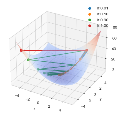
Solutions’path for different learning rates

x_range = y_range = [-5., 5.]

# Plot function surface
ax, _ = plot_surface(x_range=x_range, y_range=y_range, f=f)

# Plot solution paths
x0 = np.array([3., 4.])
lr = 0.01
weights_sol, intermediate_res = \
    gradient_descent(fun=f, x0=x0, jac=f_grad,
                     options=dict(learning_rate=lr,
                                  maxiter=10,
                                  intermediate_res=True))

sols = crop(np.array(intermediate_res["weights"]),
            x_range, y_range)
plot_path(sols[:, 0], sols[:, 1], f(sols), colors[0],
          'lr:%.02f' % lr, ax)

lr = 0.1
weights_sol, intermediate_res = \
    gradient_descent(fun=f, x0=x0, jac=f_grad,
                     options=dict(learning_rate=lr,
                                  maxiter=10,
                                  intermediate_res=True))

sols = crop(np.array(intermediate_res["weights"]),
            x_range, y_range)
plot_path(sols[:, 0], sols[:, 1], f(sols), colors[1],
          'lr:%.02f' % lr, ax)

lr = 0.9
weights_sol, intermediate_res = \
    gradient_descent(fun=f, x0=x0, jac=f_grad,
                     options=dict(learning_rate=lr,
                                  maxiter=10,
                                  intermediate_res=True))

sols = crop(np.array(intermediate_res["weights"]),
            x_range, y_range)
plot_path(sols[:, 0], sols[:, 1], f(sols), colors[2],
          'lr:%.02f' % lr, ax)

lr = 1.
weights_sol, intermediate_res = \
    gradient_descent(fun=f, x0=x0, jac=f_grad,
                     options=dict(learning_rate=lr,
                                  maxiter=10,
                                  intermediate_res=True))

sols = crop(np.array(intermediate_res["weights"]),
            x_range, y_range)
plot_path(sols[:, 0], sols[:, 1], f(sols), colors[3],
          'lr:%.02f' % lr, ax)

plt.legend()
plt.show()

Gradient Descent Numerical Approximation of the Gradient

# Numerical approximation
f_grad =  nd.Gradient(f)
print(f_grad([1, 1]))
print(f_grad([1, 2]))
print(f_grad([5, 5]))

lr = 0.1
weights_sol, intermediate_res = \
    gradient_descent(fun=f, x0=x0, jac=f_grad,
                     options=dict(learning_rate=lr,
                                  maxiter=10,
                                  intermediate_res=True))


res_ = pd.DataFrame(intermediate_res)
print(res_.head(5))
print(res_.tail(5))
print("Solution: ", weights_sol)

[3. 3.]
[4. 5.]
[15. 15.]
        eps                                   weights
0  2.210000                                [3.0, 4.0]
1  1.084500                 [2.0, 2.9000000000000203]
2  0.532701  [1.3099999999999983, 2.1200000000000156]
3  0.262073  [0.8359999999999975, 1.5650000000000128]
4  0.129266  [0.5122999999999966, 1.1684000000000108]
        eps                                      weights
5  0.064029    [0.29299999999999615, 0.8834900000000089]
6  0.031932    [0.14605099999999605, 0.6774920000000075]
7  0.016099    [0.04909159999999599, 0.5273885000000065]
8  0.008254   [-0.01346557000000384, 0.4170016400000056]
9  0.004341  [-0.05247262000000364, 0.33494786900000495]
Solution:  [-0.07547288  0.27320556]

First-order Gradient Descent to Minimize Linear Regression

Least squares problem solved by linear regression

Given a linear model where the output is a weighted sum of the inputs, the model can be expressed as:

\[y_i = \sum_p w_p x_{ip}\]

where:

• \(y_i\) is the predicted output for the i-th sample,

• \(w_p\) are the weights (parameters) of the model,

• \(x_{ip}\) is the p-th feature of the i-th sample.

The objective in least squares minimization is to minimize the following cost function \(J(\textbf{w})\):

\[J(\textbf{w}) = \frac{1}{2} \sum_i \left(y_i - \sum_p w_p x_{ip}\right)^2\]

where w is the vector of weights \(\textbf{w} = [w_1, w_2, \ldots, w_p]^T\).

Gradient vector (Jacobian) of the least squares problem solved by linear regression

Gradient of the cost function \(\nabla J(\textbf{w})\):

\[\nabla J(\textbf{w}) = \frac{\partial J(\textbf{w})}{\partial w_p} \sum_i\left(\sum_q w_q x_{iq} - y_i\right)x_{ip}.\]

Note that the gradient is also called the Jacobian which is the vector of first-order partial derivatives of a scalar-valued function of several variables.

def lse(weights, X, y):
    """
    Least Squared Error function.

    Parameters
    ----------
    weights: coefficients of the linear model, (n_features) numpy array
    X: input variables, (n_samples x n_features) numpy array
    y: target variable, (n_samples,) numpy array

    Returns
    -------
    Least Squared Error, scalar
    """

    y_pred = np.dot(X, weights)
    err = y_pred - y
    return np.sum(err ** 2)


def gradient_lse_lr(weights, X, y):
    """Gradient of Least Squared Error cost function of linear regression.

    Parameters
    ----------
    weights: coefficients of the linear model, (n_features) numpy array
    X: input variables, (n_samples x n_features) numpy array
    y: target variable, (n_samples,) numpy array

    Returns
    -------
    Gradient array, shape (n_features,)
    """
    y_pred = np.dot(X, weights)
    err = y_pred - y
    grad = np.dot(err, X)
    return grad

import numpy as np
n_sample, n_features = 100, 2
X = np.random.randn(n_sample, n_features)
weights = np.array((3, 2))
y = np.dot(X, weights)

lr = 0.01
weights_sol, intermediate_res = \
    gradient_descent(fun=lse, x0=np.zeros(weights.shape), args=(X, y),
                     jac=gradient_lse_lr,
                     options=dict(learning_rate=lr,
                                  maxiter=15,
                                  intermediate_res=True))

import pandas as pd
print(pd.DataFrame(intermediate_res))
print("Solution: ", weights_sol)

             eps                                   weights
0   1.827068e+01                                [0.0, 0.0]
1   2.533290e+00   [2.9606455406811665, 3.083060577054058]
2   5.688808e-01  [2.9474878311671824, 1.4914837597307526]
3   1.285869e-01   [3.0215058147349247, 2.242084930205261]
4   2.906710e-02    [2.989606930891622, 1.884916456416018]
5   6.570631e-03   [3.004933187739197, 2.0547169361452395]
6   1.485294e-03   [2.997654130404577, 1.9739849976431851]
7   3.357514e-04    [3.0011153188655446, 2.01236877321922]
8   7.589676e-05   [2.9994697233396193, 1.994119296045902]
9   1.715650e-05   [3.000252118741238, 2.0027959668215187]
10  3.878234e-06   [2.999880130737226, 1.9986706641729648]
11  8.766766e-07  [3.0000569915580053, 2.0006320295819435]
12  1.981731e-07   [2.9999729034982328, 1.999699503026759]
13  4.479713e-08  [3.0000128829678214, 2.0001428705768003]
14  1.012641e-08   [2.999993874823351, 1.9999320725214131]
Solution:  [3.00000291 2.0000323 ]

Second-order Newton’s method in optimization

Newton’s method integrates the change of the curvature (ie, change of gradient direction) in the minimization process. Since gradient direction is the change of \(f\), i.e., the first order derivative, thus the change of gradient is second order derivative of \(f\). See Visually Explained: Newton’s Method in Optimization

For univariate functions. Like gradient descent Newton’s method try to locally minimize \(f(w_k + t)\) given a current position \(w_k\). However, while gradient descent use first order local estimation of \(f\), Newton’s method increases this approximation using second-order Taylor expansion of \(f\) around an iterate \(w_k\):

\[f(w_k + t) \approx f(w_k) + f'(w_k)t + \frac{1}{2} f''(w_k)t^2\]

Cancelling the derivative of this expression: \(\frac{d}{dt}(f(w_k) + f'(w_k)t + \frac{1}{2} f''(w_k)t^2)=0\), provides \(f'(w_k) + f''(w_k)t = 0\), and thus \(t = \frac{f'(w_k)}{f''(w_k)}\). The learning rate is \(\gamma = \frac{1}{f''(w_k)}\), and optimization scheme becomes:

\[w_{k+1} = w_{k} - \frac{1}{f''(w_k)} f'(w_{k}).\]

In multidimensional problems \(\textbf{w}_{k} \in \mathbb{R}^p\), \([f''(\textbf{w}_k)]^{-1}\) is the inverse of the \((p \times p)\) Hessian matrix containing the second-order partial derivatives of \(f\). It is noted:

\[f''(\textbf{w}_k) = \nabla^2 f(\textbf{w}_k) = \textbf{H}_{f(\textbf{w}_k)}\]

The optimization scheme becomes:

\[\textbf{w}_{k+1} = \textbf{w}_{k} - \gamma \left[\textbf{H}_{f(\textbf{w}_k)}\right]^{-1} \nabla f(\textbf{w}_{k}).\]

We can introduce a small step size \(0 \leq \gamma < 1\) instead of \(\gamma = 1\).

• Benefit of Newton’s method: Convergence speed considering the change of the curvature of \(f\) to adapt the learning rate and direction.

• Problems:

• Local minima (local optimization) for non-convex problem.

• In large dimension, computing the Newton direction \(-[f''(w_k)]^{-1} f'(w_{k})\) can be an expensive operation.

Second-order Newton’s Method to Minimize Linear Regression

** Hessian Matrix of the Least Squares Problem solved by Linear Regression**

The Hessian matrix \(H\) of the least squares problem is a square matrix of second-order partial derivatives of the cost function with respect to the model parameters. It is given by:

\[H = \nabla^2 J(\textbf{w})\]

For the least squares cost function, \(J(\textbf{w})\), the Hessian is calculated as follows:

The Hessian \(H\) is the matrix of second derivatives of \(J(\textbf{w})\) with respect to \(w_p\) and \(w_q\). \(H\) is a measure of the curvature of \(J\): The eigenvectors of \(H\) point in the directions of the major and minor axes. The eigenvalues measure the steepness of \(J\) along the corresponding eigendirection. Thus, each eigenvalue of \(H\) is also a measure of the covariance or spread of the inputs along the corresponding eigendirection.

\[H_{pq} = \frac{\partial^2 J(\textbf{w})}{\partial w_p \partial w_q}\]

Given the form of the gradient, the second derivative with respect to \(w_p\) and \(w_q\) simplifies to:

\[H_{pq} = \sum_i x_{ip}x_{iq}\]

This can be written more compactly in matrix form as:

\[H = \textbf{X}^T\textbf{X}\]

where \(X\) is the matrix of input features (each row corresponds to a sample, and each column corresponds to a feature) with \(X_{ip}=x_{ip}\).

In this case the Hessian turns out the be the same as the covariance matrix of the inputs. Thus, each eigenvalue of \(H\) is also a measure of the covariance or spread of the inputs along the corresponding eigendirection.

def hessian_lse_lr(weights, X, y):
    """Hessian of Least Squared Error cost function of linear regression.
    To make API compatible with scipy.optimize.minimize, it takes a required weights parameters
    that is not used.

    Parameters
    ----------
    weights: coefficients of the linear model, (n_features) numpy array
    It is not used, you can safely give None.
    X: input variables, (n_samples x n_features) numpy array
    y: target variable, (n_samples,) numpy array

    Returns
    -------
    Hessian array, shape (n_features, n_features)
    """
    return np.dot(X.T, X)


weights_sol, intermediate_res = \
    gradient_descent(fun=lse, x0=np.zeros(weights.shape), args=(X, y),
                     jac=gradient_lse_lr, hess=hessian_lse_lr,
                     options=dict(learning_rate=0.01,
                                  maxiter=15,
                                  intermediate_res=True))

print(pd.DataFrame(intermediate_res))
print("Solution: ", weights_sol)

             eps                                   weights
0   1.827068e+01                                [0.0, 0.0]
1   2.533290e+00   [2.9606455406811665, 3.083060577054058]
2   5.688808e-01  [2.9474878311671824, 1.4914837597307526]
3   1.285869e-01   [3.0215058147349247, 2.242084930205261]
4   2.906710e-02    [2.989606930891622, 1.884916456416018]
5   6.570631e-03   [3.004933187739197, 2.0547169361452395]
6   1.485294e-03   [2.997654130404577, 1.9739849976431851]
7   3.357514e-04    [3.0011153188655446, 2.01236877321922]
8   7.589676e-05   [2.9994697233396193, 1.994119296045902]
9   1.715650e-05   [3.000252118741238, 2.0027959668215187]
10  3.878234e-06   [2.999880130737226, 1.9986706641729648]
11  8.766766e-07  [3.0000569915580053, 2.0006320295819435]
12  1.981731e-07   [2.9999729034982328, 1.999699503026759]
13  4.479713e-08  [3.0000128829678214, 2.0001428705768003]
14  1.012641e-08   [2.999993874823351, 1.9999320725214131]
Solution:  [3.00000291 2.0000323 ]

Quasi-Newton Methods

Quasi-Newton Methods are an alternative of Newton Methods when Hessian is unavailable or is too expensive to compute at every iteration.

The most popular quasi-Newton method is the Broyden–Fletcher–Goldfarb–Shanno algorithm BFGS

Example: Minimizes linear regression

Note, that we provide the function to be minimized (Mean Squared Error) but the expression of the gradient which is estimated numerically.

from scipy.optimize import minimize

result = minimize(fun=lse, x0=[0, 0], args=(X, y), method='BFGS')
b0, b1 = result.x

print("Solution: {:e} x + {:e}".format(b1, b0))

Solution: 2.000000e+00 x + 3.000000e+00

Gradient Descent Variants: Data Sampling Strategies

There are three variants of gradient descent, which differ on the use of the dataset made of \(n\) samples of input data \(\textbf{x}_i\)’s, and possibly their corresponding targets \(y_i\)’s.

Batch gradient descent

Batch gradient descent, known also as Vanilla gradient descent, computes the gradient of the cost function with respect to the parameters \(\theta\) for the entire training dataset :

• Choose an initial vector of parameters \(\textbf{w}_0\) and learning rate \(\gamma\).

• Repeat until an approximate minimum is obtained:

  • \(\textbf{w}_{k+1} = \textbf{w}_{k} - \gamma \sum_{i=1}^n \nabla f(\textbf{w}_{k}, \textbf{x}_i, y_i)\)

Advantages:

• Batch Gradient Descent is suited for convex or relatively smooth error manifolds. Since it directly towards an optimum solution.

Limitations:

• Fast convergence toward “bad” local minimum (on non-convex functions)

• As we need to calculate the gradients for the whole dataset is intractable for datasets that don’t fit in memory and doesn’t allow us to update our model online.

Stochastic gradient descent

Stochastic gradient descent (SGD) in contrast performs a parameter update for each training example \(x^{(i)}\) and \(y^{(i)}\). A complete passes through the training dataset is called an epoch. The number of epochs is a hyperparameter to be determined observing the convergence.

• Choose an initial vector of parameters \(\textbf{w}_0\) and learning rate \(\gamma\).

• Repeat epochs until an approximate minimum is obtained:

  • Randomly shuffle examples in the training set.

  • For \(i \in 1, \dots, n\)

    • \(\textbf{w}_{k+1} = \textbf{w}_{k} - \gamma \nabla f(\textbf{w}_{k}, \textbf{x}_i, y_i)\)

Advantages:

• Often provide better local minimum. Minimization will not be smooth but rather slightly erratic and jumpy. But this ‘random walk,’ of SGD’s fluctuation, enables it to jump from a basin to another, with possibly deeper, local minimum.

• Online learning

Limitations:

• Large fluctuation that ultimately complicates convergence to the exact minimum, as SGD will keep overshooting. However, when we slowly decrease the learning rate, SGD shows the same convergence behaviour as batch gradient descent, almost certainly converging to a local or the global minimum for non-convex and convex optimization respectively.

• Slow down computation by not taking advantage of vectorized numerical libraries.

Mini-batch gradient descent

Mini-batch gradient descent finally takes the best of both worlds and performs an update for every mini-batch (subset of) training samples:

• Divide the training set in subsets of size \(m\).

• Choose an initial vector of parameters \(\textbf{w}_0\) and learning rate \(\gamma\).

• Repeat epochs until an approximate minimum is obtained:

  • Randomly pick a mini-batch.

  • For each mini-batch \(b\)

    • \(\textbf{w}_{k+1} = \textbf{w}_{k} - \gamma \sum_{i=b}^{b+m} \nabla f(\textbf{w}_{k}, \textbf{x}_i, y_i)\)

Advantages:

• Reduces the variance of the parameter updates, which can lead to more stable convergence.

• Make use of highly optimized matrix optimizations common to state-of-the-art deep learning libraries that make computing the gradient very efficient. Common mini-batch sizes range between 50 and 256, but can vary for different applications.

Mini-batch gradient descent is typically the algorithm of choice when training a neural network.

Momentum update

Momentum and Adaptive Learning Rate Optimizers

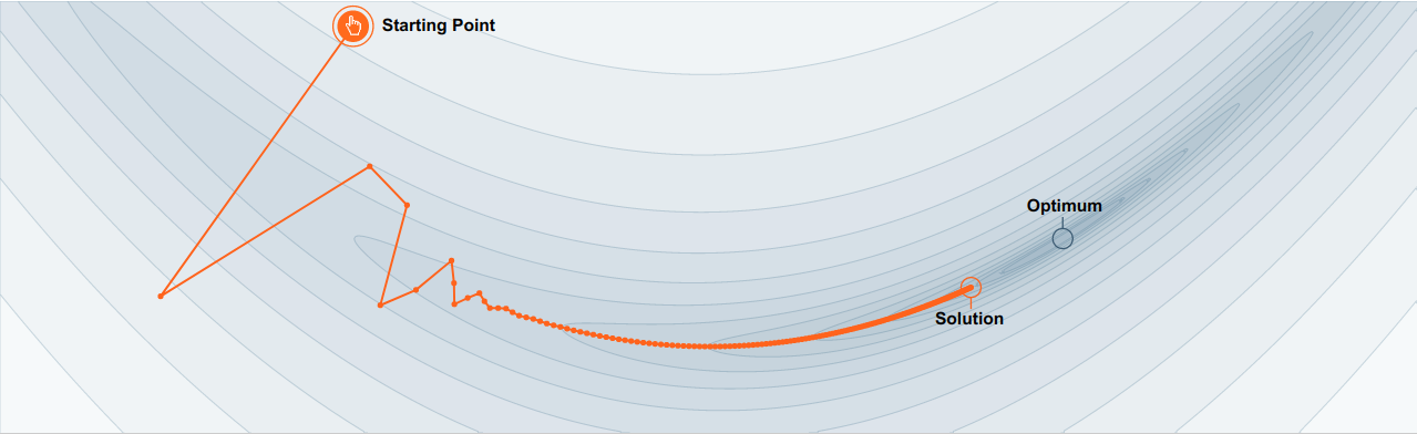
SGD has trouble navigating ravines (areas where the surface curves much more steeply in one dimension than in another), which are common around local optima. In these scenarios, SGD oscillates across the slopes of the ravine while only making hesitant progress, along the bottom towards the local optimum as in the image below.

Source

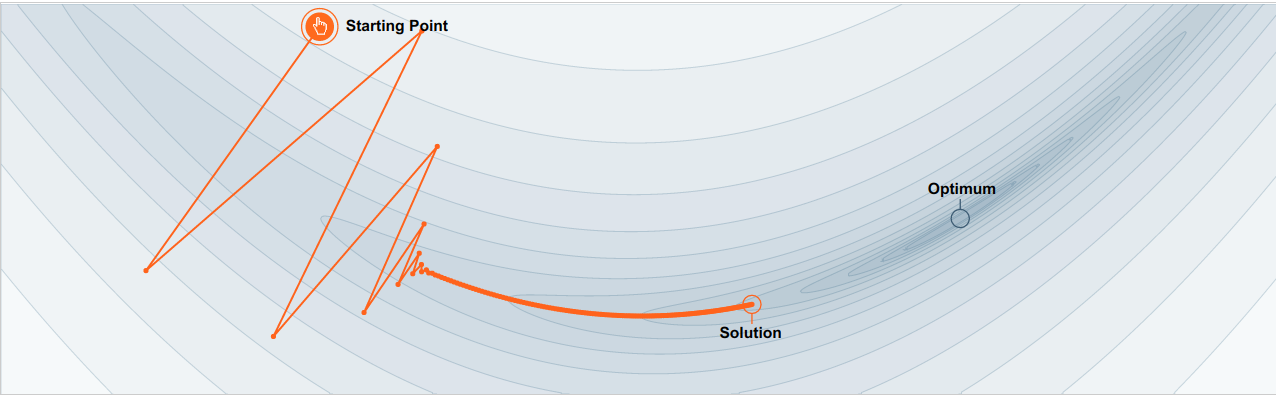
No momentum: oscillations toward local largest gradient

No momentum: moving toward local largest gradient create oscillations.

With momentum: accumulate velocity to avoid oscillations

With momentum: accumulate velocity to avoid oscillations.

Momentum is a method that helps to accelerate SGD in the relevant direction and dampens oscillations as can be seen in image above. It does this by adding a fraction \(\gamma\) of the update vector of the past time step to the current update vector.

\[\begin{split}\begin{align} \begin{split} \textbf{v}_{k+1} &= \beta \textbf{v}_{k} + \nabla J(\textbf{w}_k) \\ \textbf{w}_{k+1} &= \textbf{w}_k - \gamma \nabla \textbf{v}_{k+1} \end{split} \end{align}\end{split}\]

v = 0
while True:
    dw = gradient(J, w)
    vx = beta * v + dw
    w -= learning_rate * v

Note: The momentum term :math:`beta` is usually set to 0.9 or a similar value.

Essentially, when using momentum, we push a ball down a hill. The ball accumulates momentum as it rolls downhill, becoming faster and faster on the way, until it reaches its terminal velocity if there is air resistance, i.e. \(\beta\) <1.

The same thing happens to our parameter updates: The momentum term increases for dimensions whose gradients point in the same directions and reduces updates for dimensions whose gradients change directions. As a result, we gain faster convergence and reduced oscillation.

AdaGrad: Adaptive Learning Rates

• Added element-wise scaling of the gradient based on the historical sum of squares in each dimension.

• “Per-parameter learning rates” or “adaptive learning rates”

grad_squared = 0
while True:
    dw = gradient(J, w)
    grad_squared += dw * dw
    w -= learning_rate * dw / (np.sqrt(grad_squared) + 1e-7)

• Progress along “steep” directions is damped.

• Progress along “flat” directions is accelerated.

• Problem: step size over long time => Decays to zero.

RMSProp: “Leaky AdaGrad”

grad_squared = 0
while True:
    dw = gradient(J, w)
    grad_squared += decay_rate * grad_squared + (1 - decay_rate) * dw * dw
    w -= learning_rate * dw / (np.sqrt(grad_squared) + 1e-7)

• decay_rate = 1: gradient descent

• decay_rate = 0: AdaGrad

Nesterov accelerated gradient

However, a ball that rolls down a hill, blindly following the slope, is highly unsatisfactory. We’d like to have a smarter ball, a ball that has a notion of where it is going so that it knows to slow down before the hill slopes up again. Nesterov accelerated gradient (NAG) is a way to give our momentum term this kind of prescience. We know that we will use our momentum term \(\gamma v_{t-1}\) to move the parameters \(\theta\).

Computing \(\theta - \gamma v_{t-1}\) thus gives us an approximation of the next position of the parameters (the gradient is missing for the full update), a rough idea where our parameters are going to be. We can now effectively look ahead by calculating the gradient not w.r.t. to our current parameters \(\theta\) but w.r.t. the approximate future position of our parameters:

Again, we set the momentum term \(\gamma\) to a value of around 0.9. While Momentum first computes the current gradient and then takes a big jump in the direction of the updated accumulated gradient , NAG first makes a big jump in the direction of the previous accumulated gradient, measures the gradient and then makes a correction, which results in the complete NAG update. This anticipatory update prevents us from going too fast and results in increased responsiveness, which has significantly increased the performance of RNNs on a number of tasks

Adam

Adaptive Moment Estimation (Adam) is a method that computes adaptive learning rates for each parameter. In addition to storing an exponentially decaying average of past squared gradients :math:`v_t`, Adam also keeps an exponentially decaying average of past gradients :math:`m_t`, similar to momentum. Whereas momentum can be seen as a ball running down a slope, Adam behaves like a heavy ball with friction, which thus prefers flat minima in the error surface. We compute the decaying averages of past and past squared gradients \(\textbf{m}_t\) and \(\textbf{v}_t\) respectively as follows:

\(\textbf{m}_{t}\) and \(\textbf{v}_{t}\) are estimates of the first moment (the mean) and the second moment (the uncentered variance) of the gradients respectively, hence the name of the method. Adam (almost)

first_moment = 0
second_moment = 0
while True:
    dx = gradient(J, x)
    # Momentum:
    first_moment = beta1 * first_moment + (1 - beta1) * dx
    # AdaGrad/RMSProp
    second_moment = beta2 * second_moment + (1 - beta2) * dx * dx
    x -= learning_rate * first_moment / (np.sqrt(second_moment) + 1e-7)

As \(\textbf{m}_{t}\) and \(\textbf{v}_{t}\) are initialized as vectors of 0’s, the authors of Adam observe that they are biased towards zero, especially during the initial time steps, and especially when the decay rates are small (i.e. \(\beta_{1}\) and \(\beta_{2}\) are close to 1). They counteract these biases by computing bias-corrected first and second moment estimates:

They then use these to update the parameters (Adam update rule):

\[\theta_{t+1} = \theta_{t} - \dfrac{\eta}{\sqrt{\hat{v}_t} + \epsilon} \hat{m}_t\]

• \(\hat{m}_t\) Accumulate gradient: velocity.

• \(\hat{v}_t\) Element-wise scaling of the gradient based on the historical sum of squares in each dimension.

• Choose Adam as default optimizer

• Default values of 0.9 for \(\beta_1\), 0.999 for \(\beta_2\), and \(10^{-7}\) for \(\epsilon\).

• learning rate in a range between \(1e-3\) and \(5e-4\)

Conclusion

Sources:

• LeCun Y.A., Bottou L., Orr G.B., Müller KR. (2012) Efficient BackProp. In: Montavon G., Orr G.B., Müller KR. (eds) Neural Networks: Tricks of the Trade. Lecture Notes in Computer Science, vol 7700. Springer, Berlin, Heidelberg

• Introduction to Gradient Descent Algorithm (along with variants) in Machine Learning: Gradient Descent with Momentum, ADAGRAD and ADAM.

Summary:

• Choosing a proper learning rate can be difficult. A learning rate that is too small leads to painfully slow convergence, while a learning rate that is too large can hinder convergence and cause the loss function to fluctuate around the minimum or even to diverge.

• Learning rate schedules try to adjust the learning rate during training by e.g. annealing, i.e. reducing the learning rate according to a pre-defined schedule or when the change in objective between epochs falls below a threshold. These schedules and thresholds, however, have to be defined in advance and are thus unable to adapt to a dataset’s characteristics.

• Additionally, the same learning rate applies to all parameter updates. If our data is sparse and our features have very different frequencies, we might not want to update all of them to the same extent, but perform a larger update for rarely occurring features.

• Another key challenge of minimizing highly non-convex error functions common for neural networks is avoiding getting trapped in their numerous suboptimal local minima. These saddle points are usually surrounded by a plateau of the same error, which makes it notoriously hard for SGD to escape, as the gradient is close to zero in all dimensions.

Recommendation:

• Shuffle the examples (SGD)

• Center the input variables by subtracting the mean

• Normalize the input variable to a standard deviation of 1

• Initializing the weight

• Adaptive learning rates (momentum), using separate learning rate for each weight