Resampling and Monte Carlo Methods
Sources:
# Manipulate data
import numpy as np
import pandas as pd

# Statistics
import scipy.stats
import statsmodels.api as sm
# import statsmodels.stats.api as sms
import statsmodels.formula.api as smf
from statsmodels.stats.stattools import jarque_bera

# Plot
import matplotlib.pyplot as plt
import seaborn as sns
import pystatsml.plot_utils

# Plot parameters
plt.style.use('seaborn-v0_8-whitegrid')
fig_w, fig_h = plt.rcParams.get('figure.figsize')
plt.rcParams['figure.figsize'] = (fig_w, fig_h * .5)
colors = sns.color_palette()
Monte-Carlo simulation of Random Walk Process
One-dimensional random walk (Brownian motion)
More information: Random Walks, Central Limit Theorem
At each step \(i\) the process moves with +1 or -1 with equal probability, ie, \(X_i \in \{+1, -1\}\) with \(P(X_i=+1)=P(X_i=-1)=1/2\). Steps \(X_i\)’s are i.i.d..
Let \(S_n = \sum^n_i X_i\), or \(S_i\) (at time \(i\)) is \(S_i = S_{i-1} + X_i\)
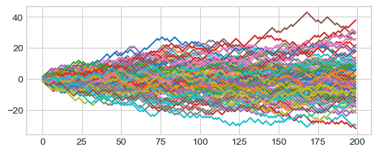
Realizations of random walks obtained by Monte Carlo simulation Plot Few random walks (trajectories), ie, \(S_n\) for \(n=0\) to \(200\)
np.random.seed(seed=42)  # make the example reproducible

n = 200  # trajectory depth
nsamp = 50000  # nb of trajectories

# X: each row (axis 0) contains one trajectory axis 1
# Xn = np.array([np.random.choice(a=[-1, +1], size=n,
#                                replace=True, p=np.ones(2) / 2)
#               for i in range(nsamp)])

Xn = np.array([np.random.choice(a=np.array([-1, +1]), size=n,
                                replace=True, p=np.ones(2)/2)
               for i in range(nsamp)])

# Sum of random walks (trajectories)
Sn = Xn.sum(axis=1)

print("True Stat. Mean={:.03f}, Sd={:.02f}".
      format(0, np.sqrt(n) * 1))

print("Est. Stat. Mean={:.03f}, Sd={:.02f}".
      format(Sn.mean(), Sn.std()))
True Stat. Mean=0.000, Sd=14.14
Est. Stat. Mean=0.010, Sd=14.09
Plot cumulative sum of 100 random walks (trajectories)
Sn_traj = Xn[:100, :].cumsum(axis=1)
_ = pd.DataFrame(Sn_traj.T).plot(legend=False)
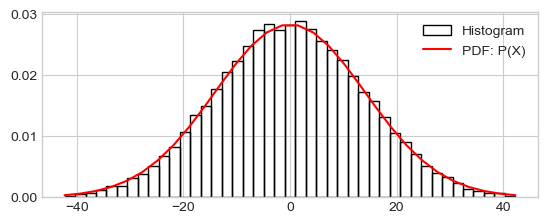
Distribution of \(S_n\) vs \(\mathcal{N}(0, \sqrt(n))\)
x_low, x_high = Sn.mean()-3*Sn.std(), Sn.mean()+3*Sn.std()
h_ = plt.hist(Sn, range=(x_low, x_high), density=True, bins=43, fill=False,
              label="Histogram")

x_range = np.linspace(x_low, x_high, 30)
prob_x_range = scipy.stats.norm.pdf(x_range, loc=Sn.mean(), scale=Sn.std())
plt.plot(x_range, prob_x_range, 'r-', label="PDF: P(X)")
_ = plt.legend()
# print(h_)
Permutation Tests
The test involves two or more samples assuming that values can be randomly permuted under the null hypothesis.
The test is Resampling procedure to estimate the distribution of a parameter or any statistic under the null hypothesis, i.e., calculated on the permuted data. This parameter or any statistic is called the estimator.
Statistical inference is conducted by computing the proportion of permuted values of the estimator that are “more extreme” than the true one, providing an estimation of the p-value.
Permutation tests are a subset of non-parametric statistics, useful when the distribution of the estimator (under H0) is unknown or requires complicated formulas.
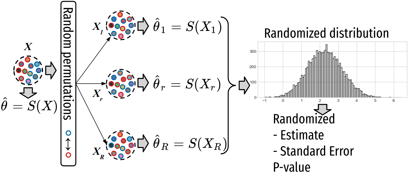
Permutation test procedure
1. Estimate the observed parameter or statistic:
on the initial dataset \(X\) of size \(N\). We call it the observed statistic.
Application to mean of one sample. Note that for genericity purposes, the proposed Python implementation can take an iterable list of arrays and calculate several statistics for several variables at once.
def mean(*x):
    return np.mean(x[0], axis=0)


# Can manage two variables, and return two statistics
x = np.array([[1, -1], [2, -2], [3, -3], [4, -4]])
print(mean(x))

# In our case with one variable
x = np.array([-1, 0, +1])
stat_obs = mean(x)
print(stat_obs)
[ 2.5 -2.5]
0.0
2. Generate B samples (called randomized samples) \([X_1, \ldots X_b, \ldots X_B]\) from the initial dataset using a adapted permutation scheme and compute the estimator (under H0):
First, we need a permutation scheme:
def onesample_sign_permutation(*x):
    """Randomly change the sign of all datsets"""
    return [np.random.choice([-1, 1], size=len(x_), replace=True) * x_
            for x_ in x]


x = np.array([-1, 0, +1])
# 10 random sign permutation of [-1, 0, +1] and mean calculation
# Mean([-1,0,1])= 0 or Mean([1,0,1])= 0.66 or Mean([-1,0,-1])= -0.66
np.random.seed(42)
stats_rnd = [float(mean(*onesample_sign_permutation(x)).round(3))
             for perm in range(10)]
print(stats_rnd)
[0.0, 0.667, 0.0, -0.667, 0.667, 0.667, 0.0, 0.667, 0.0, 0.0]
Using a parallelized permutation procedure using Joblib whose code is available here
from pystatsml import resampling

stats_rnd = np.array(resampling.resample_estimate(x, estimator=mean,
                        resample=onesample_sign_permutation, n_resamples=10))
print(stats_rnd.round(3))
[ 0. 0.667 0.667 0. 0. 0.667 0.667 -0.667 0. 0. ]
3. Permutation test: Compute statistics of the estimator under the null hypothesis using randomized estimates \(T^{(b)}\)’s.
Mean (under \(H0\)):
\[\bar{T}_B = \frac{1}{B}\sum_{b=1}^B T^{(b)}\]Standard Error \(\sigma_{T_B}\) (under \(H0\)):
\[\sigma_{T_B} = \sqrt{\frac{1}{B-1}\sum_{b=1}^B (\bar{T}_B - T^{(b)})^2}\]\(T^{(b)}\)’s provides an estimate the distribution of \(P(T | H0)\) necessary to compute p-value using the distribution (under H0):
One-sided p-value:
\[P(T \ge T^{\text{obs}} | H0) \approx \frac{\mathbf{card}(T^{(b)} \ge T^{\text{obs}})}{B}\]Two-sided p-value:
\[P(T\le T^{\text{obs}}~\text{or}~T \ge T^{\text{obs}} | H0) \approx \frac{\mathbf{card}(T^{(b)} \le T^{\text{obs}}) + \mathbf{card}(T^{(b)} \ge T^{\text{obs}})}{B}\]
Let randomized samples) \([X_1, \ldots X_r, \ldots X_rnd]\) from the initial dataset using a adapted permutation scheme and compute the estimator (under HO): \(T^{(b)} = S(X_r)\).
Permutation test: Compute statistics of the estimator under the null hypothesis using randomized estimates \(T^{(b)}\)’s.
Mean (under \(H0\)):
\[\bar{T}_B = \frac{1}{r}\sum_{r=1}^R T^{(b)}\]Standard Error \(\sigma_{T_B}\) (under \(H0\)):
\[\sigma_{T_B} = \sqrt{\frac{1}{R-1}\sum_{r=1}^K (\bar{T}_B - T^{(b)})^2}\]\(T^{(b)}\)’s provides an estimate the distribution of \(P(T | H0)\) necessary to compute p-value using the distribution (under \(H0\)):
One-sided p-value:
\[P(T\ge T^{\text{obs}} | H0) \approx \frac{\mathbf{card}(T^{(b)} \ge T^{\text{obs}})}{R}\]Two-sided p-value:
\[P(T\le T^{\text{obs}}~\text{or}~T \ge T^{\text{obs}} | H0) \approx \frac{\mathbf{card}(T^{(b)} \le T^{\text{obs}}) + \mathbf{card}(T^{(b)} \ge T^{\text{obs}})}{R}\]
# 3. Permutation test: Compute statistics under H0, estimates distribution and
# compute p-values

def permutation_test(stat_obs, stats_rnd):
    """Compute permutation test using statistic under H1 (true statistic)
    and statistics under H0 (randomized statistics) for several statistics.

    Parameters
    ----------
    stat_obs : array of shape (nb_statistics)
        statistic under H1 (true statistic)
    stats_rnd : array of shape (nb_permutations, nb_statistics)
        statistics under H0 (randomized statistics)

    Returns
    -------
    tuple
        p-value, statistics mean under HO, statistics stan under HO

    Example
    -------
    >>> np.random.seed(42)
    >>> stats_rnd = np.random.randn(1000, 5)
    >>> stat_obs = np.arange(5)
    >>> pval, stat_mean_rnd, stat_se_rnd = permutation_test(stat_obs, stats_rnd)
    >>> print(pval)
    [1.    0.315 0.049 0.002 0.   ]
    """

    n_perms = stats_rnd.shape[0]

    # 1. Randomized Statistics

    # Mean of randomized estimates
    stat_mean_rnd = np.mean(stats_rnd, axis=0)

    # Standard Error of randomized estimates
    stat_se_rnd = np.sqrt(1 / (n_perms - 1) *
                          np.sum((stat_mean_rnd - stats_rnd) ** 2, axis=0))

    # 2. Compute two-sided p-value using the distribution under H0:

    extreme_vals = (stats_rnd <= -np.abs(stat_obs)
                    ) | (stats_rnd >= np.abs(stat_obs))
    pval = np.sum(extreme_vals, axis=0) / n_perms
    # We could use:
    # (np.sum(stats_rnd <= -np.abs(stat_obs)) + \
    #  np.sum(stats_rnd >=  np.abs(stat_obs))) / n_perms

    # 3. Distribution of the parameter or statistic under H0
    # stat_density_rnd, bins = np.histogram(stats_rnd, bins=50, density=True)
    # dx = np.diff(bins)

    return pval, stat_mean_rnd, stat_se_rnd


pval, stat_mean_rnd, stat_se_rnd = permutation_test(stat_obs, stats_rnd)
print("Estimate: {:.2f}, Mean(Estimate|HO): {:.4f}, p-val: {:e}, SE: {:.3f}".
      format(stat_obs, stat_mean_rnd, pval, stat_se_rnd))
Estimate: 0.00, Mean(Estimate|HO): 0.2000, p-val: 1.000000e+00, SE: 0.450
One Sample Sign Permutation
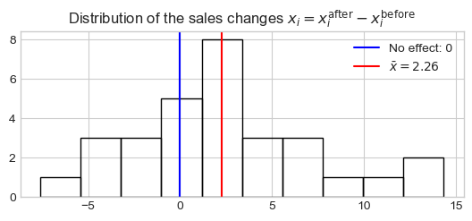
Consider the monthly revenue figures of for 100 stores before and after a marketing campaigns. We compute the difference (\(x_i = x_i^\text{after} - x_i^\text{before}\)) for each store \(i\). Under the null hypothesis, i.e., no effect of the campaigns, \(x_i^\text{after}\) and \(x_i^\text{before}\) could be permuted, which is equivalent to randomly switch the sign of \(x_i\). Here we will focus on the sample mean \(T^{\text{obs}} = S(X) = 1/n\sum_i x_i\) as statistic of interest.
Read data:
df = pd.read_csv("../datasets/Monthly Revenue (in thousands).csv")
# Reshape Keep only the 30 first samples
df = df.pivot(index='store_id', columns='time', values='revenue')[:30]
df.after -= 3  # force to smaller effect size

x = df.after - df.before

plt.hist(x, fill=False)
plt.axvline(x=0, color="b", label=r'No effect: 0')
plt.axvline(x=x.mean(), color="r", ls='-', label=r'$\bar{x}=%.2f$' % x.mean())
plt.legend()
_ = plt.title(
    r'Distribution of the sales changes $x_i = x_i^\text{after} - x_i^\text{before}$')
# 1. Estimate the observed parameter or statistic
stat_obs = mean(x)

# 2. Generate randomized samples and compute the estimator (under HO)
stats_rnd = np.array(resampling.resample_estimate(x, estimator=mean,
                        resample=onesample_sign_permutation, n_resamples=1000))

# 3. Permutation test: Compute stats. under H0, and p-values
pval, stat_mean_rnd, stat_se_rnd = permutation_test(stat_obs, stats_rnd)
print("Estimate: {:.2f}, Mean(Estimate|HO): {:.4f}, p-val: {:e}, SE: {:.3f}".
      format(stat_obs, stat_mean_rnd, pval, stat_se_rnd))
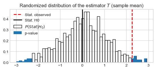
Estimate: 2.26, Mean(Estimate|HO): -0.0093, p-val: 3.900000e-02, SE: 1.051
Plot density
stats_density_rnd, bins = np.histogram(stats_rnd, bins=50, density=True)
dx = np.diff(bins)

pystatsml.plot_utils.plot_pvalue_under_h0(stat_vals=bins[1:],
                    stat_probs=stats_density_rnd,
                    stat_obs=stat_obs,  stat_h0=0, bar_width=np.diff(bins),
                    thresh_low=-np.abs(stat_obs), thresh_high=np.abs(stat_obs))
_ = plt.title(r'Randomized distribution of the estimator $T$ (sample mean)')
Similar procedure can be conducted with many statistic e.g., the t-statistic (more sensitive than the mean):
def ttest_1samp(*x):
    x = x[0]
    return (np.mean(x, axis=0) - 0) / np.std(x, ddof=1, axis=0) * np.sqrt(len(x))


# 1. Estimate the observed parameter or statistic
stat_obs = ttest_1samp(x)

# 2. Generate randomized samples and compute the estimator (under HO)
stats_rnd = np.array(resampling.resample_estimate(x, estimator=ttest_1samp,
                        resample=onesample_sign_permutation, n_resamples=1000))

# 3. Permutation test: Compute stats. under H0, and p-values
pval, stat_mean_rnd, stat_se_rnd = permutation_test(stat_obs, stats_rnd)
print("Estimate: {:.2f}, Mean(Estimate|HO): {:.4f}, p-val: {:e}, SE: {:.3f}".
      format(stat_obs, stat_mean_rnd, pval, stat_se_rnd))
Estimate: 2.36, Mean(Estimate|HO): 0.0130, p-val: 2.800000e-02, SE: 1.064
Or the median (less sensitive than the mean):
def median(*x):
    x = x[0]
    return np.median(x, axis=0)


# 1. Estimate the observed parameter or statistic
stat_obs = median(x)

# 2. Generate randomized samples and compute the estimator (under HO)
stats_rnd = np.array(resampling.resample_estimate(x, estimator=median,
                        resample=onesample_sign_permutation, n_resamples=1000))

# 3. Permutation test: Compute stats. under H0, and p-values
pval, stat_mean_rnd, stat_se_rnd = permutation_test(stat_obs, stats_rnd)
print("Estimate: {:.2f}, Mean(Estimate|HO): {:.4f}, p-val: {:e}, SE: {:.3f}".
      format(stat_obs, stat_mean_rnd, pval, stat_se_rnd))
Estimate: 1.85, Mean(Estimate|HO): 0.0255, p-val: 1.030000e-01, SE: 1.081
Two Samples Permutation
\(x\) is a variable \(y \in \{0, 1\}\) is a sample label for two groups. To obtain sample under HO we just have to permute the group’s labels \(y\):
# Dataset
from pystatsml import datasets

x, y = datasets.make_twosamples(n_samples=30, n_features=1, n_informative=1,
                                group_scale=1., noise_scale=1., shared_scale=0,
                                random_state=0)

print(scipy.stats.ttest_ind(x[y == 0], x[y == 1], equal_var=True))

# Label permutation, expect label_permutation(x, label)


def label_permutation(*x):
    x, label = x[0], x[1]
    label = np.random.permutation(label)
    return x, label


xr, yr = label_permutation(x, y)
assert np.all(x == xr)
print("Original labels:", y)
print("Permuted labels:", yr)
TtestResult(statistic=np.float64(-1.2845532458346598), pvalue=np.float64(0.2094747870423826), df=np.float64(28.0))
Original labels: [0. 0. 0. 0. 0. 0. 0. 0. 0. 0. 0. 0. 0. 0. 0. 1. 1. 1. 1. 1. 1. 1. 1. 1.
 1. 1. 1. 1. 1. 1.]
Permuted labels: [0. 1. 0. 1. 0. 0. 0. 0. 1. 1. 0. 0. 1. 0. 0. 0. 0. 1. 1. 1. 1. 0. 1. 1.
 0. 1. 1. 0. 1. 1.]
As statistic we use the student statistic of two sample test with equal variance
def twosample_ttest(*x):
    x, label = x[0], x[1]
    ttest = scipy.stats.ttest_ind(x[label == 0], x[label == 1],
                                  equal_var=True, axis=0)

    return ttest.statistic
# 1. Estimate the observed parameter or statistic
stat_obs = twosample_ttest(x, y)

# 2. Generate randomized samples and compute the estimator (under HO)

# Sequential version:
# stats_rnd = np.array([twosample_ttest(*label_permutation(x, y))
#                       for perm in range(1000)])

# Parallel version:
stats_rnd = np.array(resampling.resample_estimate(x, y, estimator=twosample_ttest,
                     resample=label_permutation, n_resamples=1000))

# 3. Permutation test: Compute stats. under H0, and p-values
pval, stat_mean_rnd, stat_se_rnd = permutation_test(stat_obs, stats_rnd)
print("Estimate: {:.2f}, Mean(Estimate|HO): {:.4f}, p-val: {:e}, SE: {:.3f}".
      format(stat_obs, stat_mean_rnd, pval, stat_se_rnd))


print("\nNon permuted t-test:")
ttest = scipy.stats.ttest_ind(x[y == 0], x[y == 1], equal_var=True)
print("Estimate: {:.2f}, p-val: {:e}".
      format(ttest.statistic, ttest.pvalue))

print("\nPermutation using scipy.stats.ttest_ind")
ttest = scipy.stats.ttest_ind(x[y == 0], x[y == 1], equal_var=True,
                              method=scipy.stats.PermutationMethod())
print("Estimate: {:.2f}, p-val: {:e}".
      format(ttest.statistic, ttest.pvalue))
Estimate: -1.28, Mean(Estimate|HO): 0.0015, p-val: 1.970000e-01, SE: 1.023

Non permuted t-test:
Estimate: -1.28, p-val: 2.094748e-01

Permutation using scipy.stats.ttest_ind
Estimate: -1.28, p-val: 1.962000e-01
Permutation-Based Correction for Multiple Testing: Westfall and Young Correction
Westfall and Young (1993) Correction for Multiple Testing, also known as maxT, controls the Family-Wise Error Rate (FWER) in the context of multiple hypothesis testing, particularly in high-dimensional settings (e.g., genomics), where traditional methods like Bonferroni are overly conservative.
The method relies on permutation testing to empirically estimate the distribution of test statistics under the global null hypothesis.
It accounts for the dependence structure between tests, improving power compared to Bonferroni-type corrections.
Procedure
Let there be \(P\) hypotheses \(H_1, \dots, H_P\) and corresponding test statistics \(T_1, \dots, T_P\):
Compute observed test statistics \(\{T_j^{\text{obs}}\}_{j=1}^P\), for each hypothesis.
Permute the data \(B\) times (e.g., shuffle labels), recomputing all \(P\) test statistics each time yielding to a \((B \times P)\) table with all permuted statistics \(\{T_j^{(b)}\}_{(b,j)}^{(B,P)}\).
For each permutation, record the maximum test statistic across all hypotheses, yielding to a vector of \(B\) maximum which value is given by:
\[M^{(b)} = \max_{j = 1, \dots, P} T_j^{(b)}\]For each hypothesis \(j\), calculate the adjusted p-value, yielding to a vector of \(P\) p-values which value is given by:
\[\tilde{p}_j = \frac{1}{B} \sum_{b=1}^B \mathbf{card}(T_j^{\text{obs}} \leq M^{(b)})\](For one-sided tests. For two-sided, take \(|T_j|\).)
Reject hypotheses with \(\tilde{p}_j \leq \alpha\).
Advantages
Strong FWER control, even under arbitrary dependence.
More powerful than Bonferroni or Holm in many dependent testing scenarios.
Non-parametric: does not rely on distributional assumptions.
Limitations
Computationally intensive, especially with large \(m\) and many permutations.
Requires exchangeability of data under the null (a key assumption for valid permutations).
Dataset
from pystatsml import datasets

n_informative = 100  # Number of features with signal (Positive features)
n_features = 1000
x, y = datasets.make_twosamples(n_samples=30, n_features=n_features, n_informative=n_informative,
                                group_scale=1., noise_scale=1., shared_scale=1.5,
                                random_state=42)
# 1. **Compute observed test statistics**
stat_obs = twosample_ttest(x, y)

# 2. Randomized statistics
stats_rnd = np.array(resampling.resample_estimate(x, y, estimator=twosample_ttest,
                     resample=label_permutation, n_resamples=1000))

def multipletests_westfall_young(stats_rnd, stat_obs):
    """Westfall and Young FWER correction for multiple comparisons.

    Parameters
    ----------
    stats_rnd : array (n_resamples, n_features)
        Randomized Statistics
    stats_true : array (n_features)
        Observed Statistics
    alpha : float, optional
        by default 0.05

    Return
    ------
    Array (n_features) P-values corrected for multiple comparison
    """

    # 3. **For each permutation**, record the **maximum test statistic**
    stat_rnd_max = np.max(np.abs(stats_rnd), axis=1)

    # 4. For each hypothesis $j$, calculate the adjusted p-value
    pvalues_ws = np.array([np.sum(stat_rnd_max >= np.abs(
        stat)) / stat_rnd_max.shape[0] for stat in stat_obs])

    return pvalues_ws

pvalues_ws = multipletests_westfall_young(stats_rnd, stat_obs)
Compute p-values using:
Un-corrected p-values: High false positives rate.
Bonferroni correction: Reduced sensitivity (low True positives rate).
Westfall and Young correction: Improved sensitivity with controlled false positive:
# Usual t-test with uncorrected p-values:
import statsmodels.sandbox.stats.multicomp as multicomp
ttest = scipy.stats.ttest_ind(x[y == 0], x[y == 1], equal_var=True)

# Classical Bonferroni correction
_, pvals_bonf, _, _ = multicomp.multipletests(ttest.pvalue, alpha=0.05,
                                              method='bonferroni')

def print_positve(title, pvalues, n_informative, n_features):
    print('%s \nPositive: %i/%i, True Positive: %i/%i, False Positive: %i/%i' %
          (title,
           np.sum(pvalues <= 0.05), n_features,
           np.sum(pvalues[:n_informative] <= 0.05), n_informative,
           np.sum(pvalues[n_informative:] <= 0.05), (n_features-n_informative)))

print_positve("No correction", ttest.pvalue, n_informative, n_features)
print_positve("Bonferroni correction", pvals_bonf, n_informative, n_features)
print_positve("Westfall and Young", pvalues_ws, n_informative, n_features)
No correction
Positive: 209/1000, True Positive: 94/100, False Positive: 115/900
Bonferroni correction
Positive: 0/1000, True Positive: 0/100, False Positive: 0/900
Westfall and Young
Positive: 4/1000, True Positive: 4/100, False Positive: 0/900
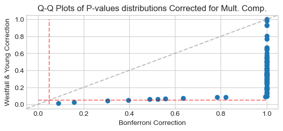
Compare P-Values distribution with Bonferroni correction for multiple comparison:
from scipy import stats
_, q_bonferroni = stats.probplot(pvals_bonf[:n_informative], fit=False)
_, q_ws = stats.probplot(pvalues_ws[:n_informative], fit=False)
ax = plt.scatter(q_bonferroni, q_ws, marker='o', color=colors[0])
ax = plt.axline([0, 0], slope=1, color="gray", ls='--', alpha=0.5)
ax = plt.vlines(0.05, 0, 1, color="r", ls='--', alpha=0.5)
ax = plt.hlines(0.05, 0, 1, color="r", ls='--', alpha=0.5)
ax = plt.xlabel('Bonferroni Correction')
ax = plt.ylabel('Westfall & Young Correction')
ax = plt.title('Q-Q Plots of P-values distributions Corrected for Mult. Comp.')
Bootstrapping
Resampling procedure to estimate the distribution of a statistic or parameter of interest, called the estimator.
Derive estimates of variability for estimator (bias, standard error, confidence intervals, etc.).
Statistical inference is conducted by looking the confidence interval (CI) contains the null hypothesis.
Nonparametric approach statistical inference, useful when model assumptions is in doubt, unknown or requires complicated formulas.
Bootstrapping with replacement has favorable performances (Efron 1979, and 1986) compared to prior methods like the jackknife that sample without replacement
Regularize models by fitting several models on bootstrap samples and averaging their predictions (see Baging and random-forest). See machine learning chapter.
Note that compared to random permutation, bootstrapping sample the distribution under the alternative hypothesis, it doesn’t consider the distribution under the null hypothesis. A great advantage of bootstrap is its simplicity of the procedure:
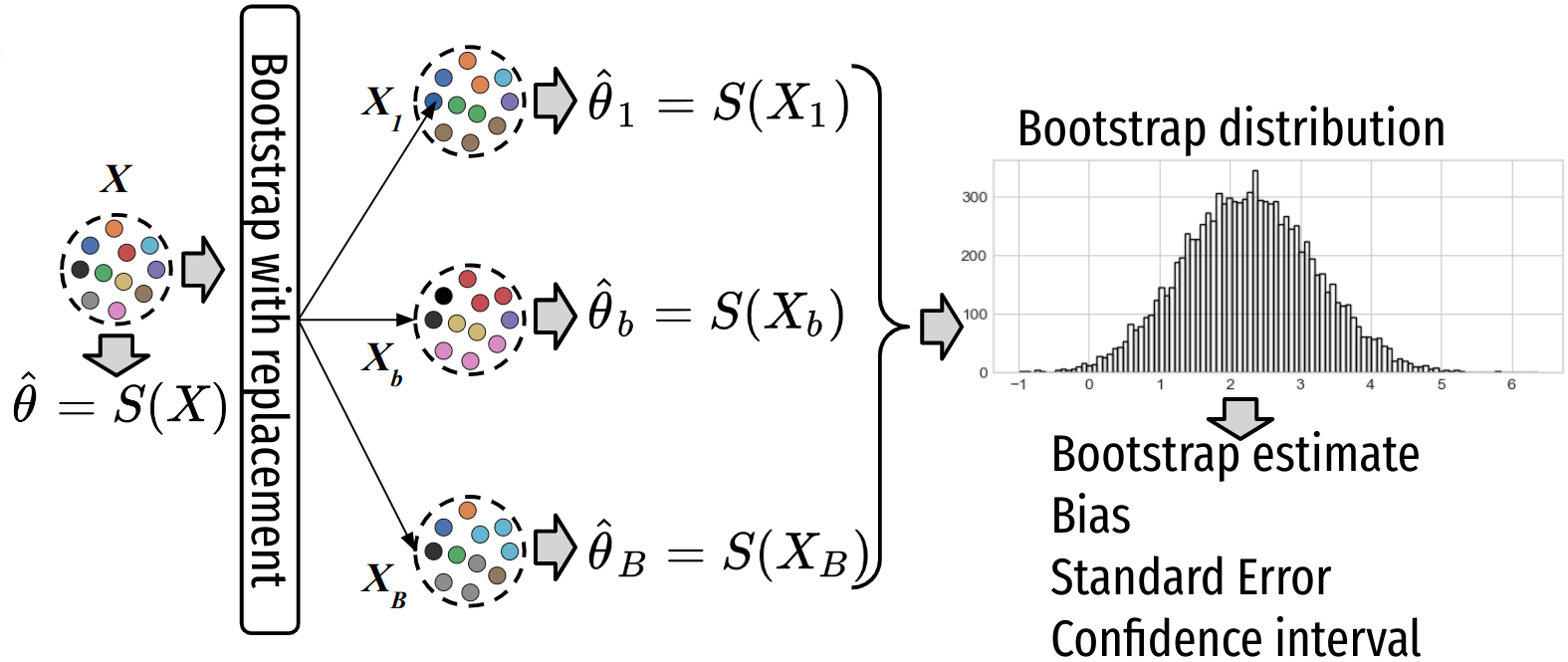
Bootstrapping procedure
Compute the estimator \(T^{\text{obs}} = S(X)\) on the initial dataset \(X\) of size \(N\).
Generate \(B\) samples (called bootstrap samples) \([X_1, \ldots X_b, \ldots X_B]\) from the initial dataset by randomly drawing with replacement $ of the N$ observations.
For each sample \(b\) compute the estimator \(\{T^{(b)}= S(X_b)\}_{b=1}^B\), which provides the bootstrap distribution \(P(T_B|H1)\) of the estimator (under the alternative hypothesis H1).
Compute statistics of the estimator on bootstrap estimates \(T^{(b)}\)’s:
Bootstrap estimate (of the parameters):
\[\bar{T_B} = \frac{1}{B}\sum_{b=1}^B T^{(b)}\]Bias = bootstrap estimate - estimate:
\[\hat{b_{T_B}} = \bar{T}_B - T^{\text{obs}}\]Standard error \(\hat{\sigma_{T_B}}\):
\[\hat{\sigma_{T_B}} = \sqrt{\frac{1}{B-1}\sum_{b=1}^B (\bar{T_B} - T^{(b)})^2}\]Confidence interval using the estimated bootstrapped distribution of the estimator:
Application using the monthly revenue of 100 stores before and after a marketing campaigns, using the difference (\(x_i = x_i^\text{after} - x_i^\text{before}\)) for each store \(i\). If the average difference \(\bar{x}=1/n \sum_i x_i\) is positive (resp. negative), then the marketing campaigns will be considered as efficient (resp. detrimental). We will use bootstrapping to compute the confidence interval (CI) and see if 0 in comprised in the CI.
x = df.after - df.before
S = np.mean

# 1. Model parameters
stat_hat = S(x)

np.random.seed(15)  # set the seed for reproducible results
B = 1000  # Number of bootstrap

# 2. Bootstrapped samples

x_B = [np.random.choice(x, size=len(x), replace=True) for boot_i in range(B)]

# 3. Bootstrap estimates and distribution

stat_hats_B = np.array([S(x_b) for x_b in x_B])
stat_density_B, bins = np.histogram(stat_hats_B, bins=50, density=True)
dx = np.diff(bins)

# 4. Bootstrap Statistics

# Bootstrap estimate
stat_bar_B = np.mean(stat_hats_B)

# Bias = bootstrap estimate - estimate
bias_hat_B = stat_bar_B - stat_hat

# Standard Error
se_hat_B = np.sqrt(1 / (B - 1) * np.sum((stat_bar_B - stat_hats_B) ** 2))

# Confidence interval using the estimated bootstrapped distribution of estimator

ci95 = np.quantile(a=stat_hats_B, q=[0.025, 0.975])

print(
    "Est.: {:.2f}, Boot Est.: {:.2f}, bias: {:e},\
     Boot SE: {:.2f}, CI: [{:.5f}, {:.5f}]"
    .format(stat_hat, stat_bar_B, bias_hat_B, se_hat_B, ci95[0], ci95[1]))
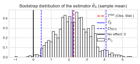
Est.: 2.26, Boot Est.: 2.19, bias: -7.201946e-02, Boot SE: 0.95, CI: [0.45256, 4.08465]
Conclusion: Zero is outside the CI, moreover \(\bar{X}\) is positive. Thus we can conclude the marketing campaign produced a significant increase of the sales.
Plot
plt.bar(bins[1:], stat_density_B, width=dx, fill=False, label=r'$P_{T_B}$')
plt.axvline(x=stat_hat, color='r', ls='--', lw=2,
            label=r'$T^{\text{obs}}$ (Obs. Stat.)')
plt.axvline(x=stat_bar_B, color="b", ls='-', label=r'$\bar{T_B}$')
plt.axvline(x=ci95[0], color="b", ls='--', label=r'$CI_{95\%}$')
plt.axvline(x=ci95[1], color="b", ls='--')
plt.axvline(x=0, color="k", lw=2, label=r'No effect: 0')
plt.legend()
_ = plt.title(
    r'Bootstrap distribution of the estimator $\hat{\theta}_b$ (sample mean)')