Multivariate Statistics¶

Multivariate statistics includes all statistical techniques for analyzing samples made of two or more variables. The data set (a \(N \times P\) matrix \(\mathbf{X}\)) is a collection of \(N\) points (or observations) with \(P\) variables, i.e., in a \(P\)-dimensional space:

\[\begin{split}\mathbf{X} = \begin{bmatrix} x_{11} & \cdots & x_{1j} & \cdots & x_{1P} \\ \vdots & & \vdots & & \vdots \\ x_{i1} & \cdots & x_{ij} & \cdots & x_{iP} \\ \vdots & & \vdots & & \vdots \\ x_{N1} & \cdots & x_{Nj} & \cdots & x_{NP} \end{bmatrix} = \begin{bmatrix} x_{11} & \ldots & x_{1P} \\ \vdots & & \vdots \\ & \mathbf{X} & \\ \vdots & & \vdots \\ x_{N1} & \ldots & x_{NP} \end{bmatrix}_{N \times P}.\end{split}\]

,

Each row \(i\) is a \(P\)-dimensional vector of the coordinates of the \(i\)’th observation or point.
Each column \(j\) is a \(N\)-dimensional vector of values of the points for the \(j\)’th variable.

Basic Linear Algebra¶

The Euclidean norm of a vector \(\mathbf{x} \in \mathbb{R}^P\) is denoted

\[\|\mathbf{x}\|_2 = \sqrt{\sum_i^P {x_i}^2}\]

The Euclidean distance between two point \(\mathbf{x}, \mathbf{y} \in \mathbb{R}^P\) is

\[\|\mathbf{x}-\mathbf{y}\|_2 = \sqrt{\sum_i^P (x_i-y_i)^2}\]

The dot product, denoted ’‘\(\cdot\)’’ of two \(P\)-dimensional vectors \(\mathbf{x} = [x_1, x_2, ..., x_P]\) and \(\mathbf{y} = [y_1, y_2, ..., y_P]\) is defined as

\[\begin{split}\mathbf{x} \cdot \mathbf{y} = \mathbf{x}^T \mathbf{y} = \sum_i x_i y_i = \begin{bmatrix} x_{1} & \ldots & \mathbf{x}^T & \ldots & x_{P} \end{bmatrix} \begin{bmatrix} y_{1}\\ \vdots \\ \mathbf{y}\\ \vdots\\ y_{P} \end{bmatrix}.\end{split}\]

Note that the Euclidean norm of a vector is the square root of the dot product of the vector with itself:

\[\left\|\mathbf{x} \right\|_2 = {\sqrt {\mathbf{x} \cdot \mathbf{x}}}.\]

Geometric interpretation: In Euclidean space, a Euclidean vector is a geometrical object that possesses both a norm (magnitude) and a direction. A vector can be pictured as an arrow. Its magnitude is its length, and its direction is the direction that the arrow points. The norm of a vector \(\mathbf{x}\) is denoted by \(\|\mathbf{x}\|_2\). The dot product of two Euclidean vectors \(\mathbf{x}\) and \(\mathbf{y}\) is defined by

\[\mathbf{x} \cdot \mathbf{y} = \|\mathbf{x} \|_2\ \|\mathbf{y} \|_2\cos \theta,\]

where \(\theta\) is the angle between \(\mathbf{x}\) and \(\mathbf{y}\).

In particular, if \(\mathbf{x}\) and \(\mathbf{y}\) are orthogonal, then the angle between them is 90° and \(\mathbf{x} \cdot \mathbf{y} = 0.\) At the other extreme, if they are codirectional, then the angle between them is 0° and \(\mathbf{x} \cdot \mathbf{y} = \left\|\mathbf{x} \right\|_2\,\left\|\mathbf{y} \right\|_2\).

The (scalar) projection of a vector \(\mathbf{x}\) (a point) in the direction of \(\mathbf{v}\) is given by

where \(\theta\) is the angle between \(\mathbf{x}\) and \(\mathbf{y}\). Note that \(x_{v}\) is a scalar measuring the length of \(x\) projected on \(v\).

When we want to project on direction \(\mathbf{v}\), we only care about its direction. Therefore vector \(\mathbf{v}\) can be normalized to \(\|\mathbf{v}\|_2 = 1\) dividing by the vector norm (without affecting its direction.). With \(\|\mathbf{v}\|_2 = 1\) the projection of any point \(\mathbf{x}\) toward a direction \(\mathbf{v}\) becomes an simple dot product:

\[x_{v} = \mathbf{x} \cdot \mathbf{v}\]

Projection of point :math:`x` on vector :math:`v` — Projection of point \(x\) on vector \(v\)¶

import numpy as np
import scipy
import pandas as pd

# Plot
import matplotlib.pyplot as plt
from matplotlib import cm # color map
import seaborn as sns
import pystatsml.plot_utils

# Plot parameters
plt.style.use('seaborn-v0_8-whitegrid')
fig_w, fig_h = plt.rcParams.get('figure.figsize')
plt.rcParams['figure.figsize'] = (fig_w, fig_h * 1.)
colors = plt.rcParams['axes.prop_cycle'].by_key()['color']

import numpy as np
np.random.seed(42)

a = np.random.randn(10)
b = np.random.randn(10)

print(np.dot(a, b))

-4.085788532659923

Mean vector¶

The mean (\(P \times 1\)) column-vector \(\mathbf{\mu}\) whose estimator is

\[\begin{split}\bar{\mathbf{x}} = \frac{1}{N}\sum_{i=1}^N \mathbf{x_i} = \frac{1}{N}\sum_{i=1}^N \begin{bmatrix} x_{i1}\\ \vdots\\ x_{ij}\\ \vdots\\ x_{iP}\\ \end{bmatrix} = \begin{bmatrix} \bar{x}_{1}\\ \vdots\\ \bar{x}_{j}\\ \vdots\\ \bar{x}_{P}\\ \end{bmatrix}.\end{split}\]

Covariance matrix¶

The covariance matrix \(\mathbf{\Sigma_{XX}}\) is a symmetric positive semi-definite matrix whose element in the \(j, k\) position is the covariance between the \(j^{th}\) and \(k^{th}\) elements of a random vector i.e. the \(j^{th}\) and \(k^{th}\) columns of \(\mathbf{X}\).
The covariance matrix generalizes the notion of covariance to multiple dimensions.
The covariance matrix describe the shape of the sample distribution around the mean assuming an elliptical distribution:

\[\mathbf{\Sigma_{XX}} = E(\mathbf{X}-E(\mathbf{X}))^TE(\mathbf{X}-E(\mathbf{X})),\]

whose estimator \(\mathbf{S_{XX}}\) is a \(P \times P\) matrix given by

\[\mathbf{S_{XX}}= \frac{1}{N-1}(\mathbf{X}- \mathbf{1} \bar{\mathbf{x}}^T)^T (\mathbf{X}- \mathbf{1} \bar{\mathbf{x}}^T).\]

If we assume that \(\mathbf{X}\) is centered, i.e. \(\mathbf{X}\) is replaced by \(\mathbf{X} - \mathbf{1}\bar{\mathbf{x}}^T\) then the estimator is

\[\begin{split}\mathbf{S_{XX}} = \frac{1}{N-1} \mathbf{X}^T\mathbf{X} = \frac{1}{N-1} \begin{bmatrix} x_{11} & \cdots & x_{N1} \\ x_{1j} & \cdots & x_{Nj} \\ \vdots & & \vdots \\ x_{1P} & \cdots & x_{NP} \\ \end{bmatrix} \begin{bmatrix} x_{11} & \cdots & x_{1k}& x_{1P}\\ \vdots & & \vdots & \vdots\\ x_{N1} & \cdots & x_{Nk}& x_{NP} \end{bmatrix}= \begin{bmatrix} s_{1} & \ldots & s_{1k} & s_{1P}\\ & \ddots & s_{jk} & \vdots\\ & & s_{k} & s_{kP}\\ & & & s_{P}\\ \end{bmatrix},\end{split}\]

where

\[s_{jk} = s_{kj} = \frac{1}{N-1} \mathbf{x_j}^T \mathbf{x_k} = \frac{1}{N-1} \sum_{i=1}^N x_{ij} x_{ik}\]

is an estimator of the covariance between the \(j^{th}\) and \(k^{th}\) variables.

np.random.seed(42)
colors = sns.color_palette()

n_samples, n_features = 100, 2

mean, Cov, X = [None] * 4, [None] * 4, [None] * 4
mean[0] = np.array([-2.5, 2.5])
Cov[0] = np.array([[1, 0],
                   [0, 1]])

mean[1] = np.array([2.5, 2.5])
Cov[1] = np.array([[1, .5],
                   [.5, 1]])

mean[2] = np.array([-2.5, -2.5])
Cov[2] = np.array([[1, .9],
                   [.9, 1]])

mean[3] = np.array([2.5, -2.5])
Cov[3] = np.array([[1, -.9],
                   [-.9, 1]])

# Generate dataset
for i in range(len(mean)):
    X[i] = np.random.multivariate_normal(mean[i], Cov[i], n_samples)

# Plot
for i in range(len(mean)):
    # Points
    plt.scatter(X[i][:, 0], X[i][:, 1], color=colors[i], label="class %i" % i)
    # Means
    plt.scatter(mean[i][0], mean[i][1], marker="o", s=200, facecolors='w',
                edgecolors=colors[i], linewidth=2)
    # Ellipses representing the covariance matrices
    pystatsml.plot_utils.plot_cov_ellipse(Cov[i], pos=mean[i], facecolor='none',
                                          linewidth=2, edgecolor=colors[i])

plt.axis('equal')
_ = plt.legend(loc='upper left')

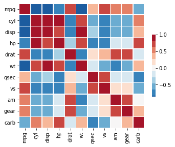
Correlation matrix¶

url = 'https://raw.githubusercontent.com/plotly/datasets/master/mtcars.csv'
df = pd.read_csv(url)
df = df.drop('manufacturer', axis=1)

# Compute the correlation matrix
corr = df.corr()

# Generate a mask for the upper triangle
mask = np.zeros_like(corr, dtype=np.bool)
mask[np.triu_indices_from(mask)] = True

f, ax = plt.subplots(figsize=(5.5, 4.5))
cmap = sns.color_palette("RdBu_r", 11)
# Draw the heatmap with the mask and correct aspect ratio
_ = sns.heatmap(corr, mask=None, cmap=cmap, vmax=1, center=0,
            square=True, linewidths=.5, cbar_kws={"shrink": .5})

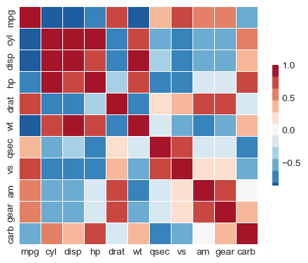
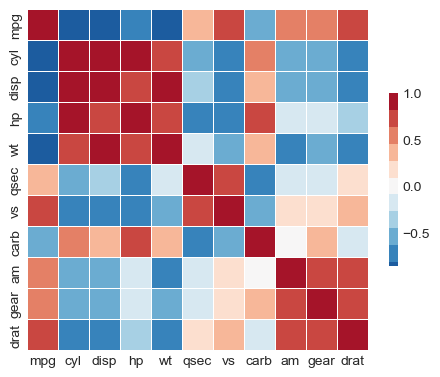
Re-order correlation matrix using AgglomerativeClustering

# convert correlation to distances
from sklearn.cluster import AgglomerativeClustering
d = 2 * (1 - np.abs(corr))

clustering = AgglomerativeClustering(
    n_clusters=3, linkage='single', metric="precomputed").fit(d)
lab = 0

clusters = [list(corr.columns[clustering.labels_ == lab])
            for lab in set(clustering.labels_)]
print(clusters)

reordered = np.concatenate(clusters)

R = corr.loc[reordered, reordered]

f, ax = plt.subplots(figsize=(5.5, 4.5))
# Draw the heatmap with the mask and correct aspect ratio
_ = sns.heatmap(R, mask=None, cmap=cmap, vmax=1, center=0,
                square=True, linewidths=.5, cbar_kws={"shrink": .5})

[['mpg', 'cyl', 'disp', 'hp', 'wt', 'qsec', 'vs', 'carb'], ['am', 'gear'], ['drat']]

Precision matrix¶

In statistics, precision is the reciprocal of the variance, and the precision matrix is the matrix inverse of the covariance matrix.

It is related to partial correlations that measures the degree of association between two variables, while controlling the effect of other variables.

import numpy as np

Cov = np.array([[1.0, 0.9, 0.9, 0.0, 0.0, 0.0],
                [0.9, 1.0, 0.9, 0.0, 0.0, 0.0],
                [0.9, 0.9, 1.0, 0.0, 0.0, 0.0],
                [0.0, 0.0, 0.0, 1.0, 0.9, 0.0],
                [0.0, 0.0, 0.0, 0.9, 1.0, 0.0],
                [0.0, 0.0, 0.0, 0.0, 0.0, 1.0]])

print("# Precision matrix:")
Prec = np.linalg.inv(Cov)
print(Prec.round(2))

print("# Partial correlations:")
Pcor = np.zeros(Prec.shape)
Pcor[::] = np.nan

for i, j in zip(*np.triu_indices_from(Prec, 1)):
    Pcor[i, j] = - Prec[i, j] / np.sqrt(Prec[i, i] * Prec[j, j])

print(Pcor.round(2))

# Precision matrix:
[[ 6.79 -3.21 -3.21  0.    0.    0.  ]
 [-3.21  6.79 -3.21  0.    0.    0.  ]
 [-3.21 -3.21  6.79  0.    0.    0.  ]
 [ 0.    0.    0.    5.26 -4.74  0.  ]
 [ 0.    0.    0.   -4.74  5.26  0.  ]
 [ 0.    0.    0.    0.    0.    1.  ]]
# Partial correlations:
[[  nan  0.47  0.47 -0.   -0.   -0.  ]
 [  nan   nan  0.47 -0.   -0.   -0.  ]
 [  nan   nan   nan -0.   -0.   -0.  ]
 [  nan   nan   nan   nan  0.9  -0.  ]
 [  nan   nan   nan   nan   nan -0.  ]
 [  nan   nan   nan   nan   nan   nan]]

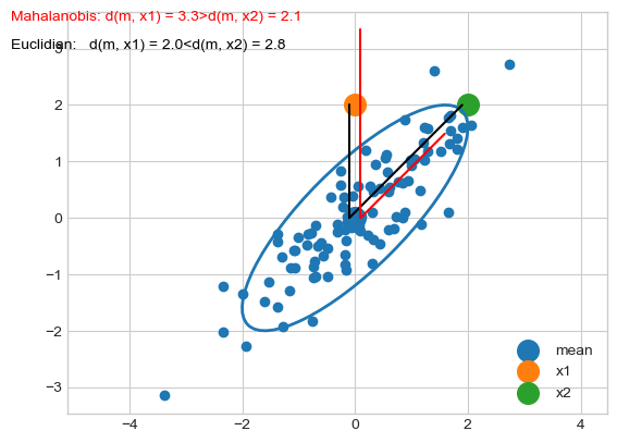
Mahalanobis distance¶

The Mahalanobis distance is a measure of the distance between two points \(\mathbf{x}\) and \(\mathbf{\mu}\) where the dispersion (i.e. the covariance structure) of the samples is taken into account.
The dispersion is considered through covariance matrix.

This is formally expressed as

\[D_M(\mathbf{x}, \mathbf{\mu}) = \sqrt{(\mathbf{x} - \mathbf{\mu})^T \mathbf{\Sigma}^{-1}(\mathbf{x} - \mathbf{\mu})}.\]

Intuitions

Distances along the principal directions of dispersion are contracted since they correspond to likely dispersion of points.
Distances othogonal to the principal directions of dispersion are dilated since they correspond to unlikely dispersion of points.

For example

\[D_M(\mathbf{1}) = \sqrt{\mathbf{1}^T \mathbf{\Sigma}^{-1}\mathbf{1}}.\]

ones = np.ones(Cov.shape[0])
d_euc = np.sqrt(np.dot(ones, ones))
d_mah = np.sqrt(np.dot(np.dot(ones, Prec), ones))

print("Euclidean norm of ones=%.2f. Mahalanobis norm of ones=%.2f" %
      (d_euc, d_mah))

Euclidean norm of ones=2.45. Mahalanobis norm of ones=1.77

The first dot product that distances along the principal directions of dispersion are contracted:

print(np.dot(ones, Prec))

[0.35714286 0.35714286 0.35714286 0.52631579 0.52631579 1.        ]

import numpy as np
import scipy
import matplotlib.pyplot as plt
import seaborn as sns
import pystatsml.plot_utils
%matplotlib inline
np.random.seed(40)
colors = sns.color_palette()

mean = np.array([0, 0])
Cov = np.array([[1, .8],
                [.8, 1]])
samples = np.random.multivariate_normal(mean, Cov, 100)
x1 = np.array([0, 2])
x2 = np.array([2, 2])

plt.scatter(samples[:, 0], samples[:, 1], color=colors[0])
plt.scatter(mean[0], mean[1], color=colors[0], s=200, label="mean")
plt.scatter(x1[0], x1[1], color=colors[1], s=200, label="x1")
plt.scatter(x2[0], x2[1], color=colors[2], s=200, label="x2")

# plot covariance ellipsis
pystatsml.plot_utils.plot_cov_ellipse(Cov, pos=mean, facecolor='none',
                                      linewidth=2, edgecolor=colors[0])
# Compute distances
d2_m_x1 = scipy.spatial.distance.euclidean(mean, x1)
d2_m_x2 = scipy.spatial.distance.euclidean(mean, x2)

Covi = scipy.linalg.inv(Cov)
dm_m_x1 = scipy.spatial.distance.mahalanobis(mean, x1, Covi)
dm_m_x2 = scipy.spatial.distance.mahalanobis(mean, x2, Covi)

# Plot distances
vm_x1 = (x1 - mean) / d2_m_x1
vm_x2 = (x2 - mean) / d2_m_x2
jitter = .1
plt.plot([mean[0] - jitter, d2_m_x1 * vm_x1[0] - jitter],
         [mean[1], d2_m_x1 * vm_x1[1]], color='k')
plt.plot([mean[0] - jitter, d2_m_x2 * vm_x2[0] - jitter],
         [mean[1], d2_m_x2 * vm_x2[1]], color='k')

plt.plot([mean[0] + jitter, dm_m_x1 * vm_x1[0] + jitter],
         [mean[1], dm_m_x1 * vm_x1[1]], color='r')
plt.plot([mean[0] + jitter, dm_m_x2 * vm_x2[0] + jitter],
         [mean[1], dm_m_x2 * vm_x2[1]], color='r')

plt.legend(loc='lower right')
plt.text(-6.1, 3,
         'Euclidian:   d(m, x1) = %.1f<d(m, x2) = %.1f' % (d2_m_x1, d2_m_x2),
         color='k')
plt.text(-6.1, 3.5,
         'Mahalanobis: d(m, x1) = %.1f>d(m, x2) = %.1f' % (dm_m_x1, dm_m_x2),
         color='r')

plt.axis('equal')
print('Euclidian   d(m, x1) = %.2f < d(m, x2) = %.2f' % (d2_m_x1, d2_m_x2))
print('Mahalanobis d(m, x1) = %.2f > d(m, x2) = %.2f' % (dm_m_x1, dm_m_x2))

Euclidian   d(m, x1) = 2.00 < d(m, x2) = 2.83
Mahalanobis d(m, x1) = 3.33 > d(m, x2) = 2.11

If the covariance matrix is the identity matrix, the Mahalanobis distance reduces to the Euclidean distance. If the covariance matrix is diagonal, then the resulting distance measure is called a normalized Euclidean distance.

More generally, the Mahalanobis distance is a measure of the distance between a point \(\mathbf{x}\) and a distribution \(\mathcal{N}(\mathbf{x}|\mathbf{\mu}, \mathbf{\Sigma})\). It is a multi-dimensional generalization of the idea of measuring how many standard deviations away \(\mathbf{x}\) is from the mean. This distance is zero if \(\mathbf{x}\) is at the mean, and grows as \(\mathbf{x}\) moves away from the mean: along each principal component axis, it measures the number of standard deviations from \(\mathbf{x}\) to the mean of the distribution.

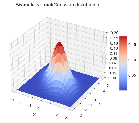
Multivariate normal distribution¶

The distribution, or probability density function (PDF) (sometimes just density), of a continuous random variable is a function that describes the relative likelihood for this random variable to take on a given value.

The multivariate normal distribution, or multivariate Gaussian distribution, of a \(P\)-dimensional random vector \(\mathbf{x} = [x_1, x_2, \ldots, x_P]^T\) is

\[\mathcal{N}(\mathbf{x}|\mathbf{\mu}, \mathbf{\Sigma}) = \frac{1}{(2\pi)^{P/2}|\mathbf{\Sigma}|^{1/2}}\exp\{-\frac{1}{2} (\mathbf{x} - \mathbf{\mu)}^T \mathbf{\Sigma}^{-1}(\mathbf{x} - \mathbf{\mu})\}.\]

import numpy as np
import matplotlib.pyplot as plt
import scipy.stats
from scipy.stats import multivariate_normal
#from mpl_toolkits.mplot3d import Axes3D


def multivariate_normal_pdf(X, mean, sigma):
    """Multivariate normal probability density function over X
    (n_samples x n_features)"""
    P = X.shape[1]
    det = np.linalg.det(sigma)
    norm_const = 1.0 / (((2*np.pi) ** (P/2)) * np.sqrt(det))
    X_mu = X - mu
    inv = np.linalg.inv(sigma)
    d2 = np.sum(np.dot(X_mu, inv) * X_mu, axis=1)
    return norm_const * np.exp(-0.5 * d2)

# mean and covariance
mu = np.array([0, 0])
sigma = np.array([[1, -.5],
                  [-.5, 1]])

# x, y grid
x, y = np.mgrid[-3:3:.1, -3:3:.1]
X = np.stack((x.ravel(), y.ravel())).T
norm = multivariate_normal_pdf(X, mean, sigma).reshape(x.shape)

# Do it with scipy
norm_scpy = multivariate_normal(mu, sigma).pdf(np.stack((x, y), axis=2))
assert np.allclose(norm, norm_scpy)

# Plot
fig, ax = plt.subplots(subplot_kw={"projection": "3d"})
surf = ax.plot_surface(x, y, norm, rstride=3,
        cstride=3, cmap=plt.cm.coolwarm,
        linewidth=1, antialiased=False
    )

ax.set_zlim(0, 0.2)
ax.zaxis.set_major_locator(plt.LinearLocator(10))
ax.zaxis.set_major_formatter(plt.FormatStrFormatter('%.02f'))

ax.set_xlabel('X')
ax.set_ylabel('Y')
ax.set_zlabel('p(x)')

plt.title('Bivariate Normal/Gaussian distribution')
fig.colorbar(surf, shrink=0.5, aspect=7, cmap=plt.cm.coolwarm)
plt.show()

Exercises¶

Dot product and Euclidean norm¶

Given \(\mathbf{x} = [2, 1]^T\) and \(\mathbf{y} = [1, 1]^T\)

Write a function euclidean(x) that computes the Euclidean norm of vector, \(\mathbf{x}\).
Compute the Euclidean norm of \(\mathbf{x}\).
Compute the Euclidean distance of \(\|\mathbf{x}-\mathbf{y}\|_2\).
Compute the projection of \(\mathbf{y}\) in the direction of vector \(\mathbf{x}\): \(y_{a}\).
Simulate a dataset \(\mathbf{X}\) of \(N=100\) samples of 2-dimensional vectors.
Project all samples in the direction of the vector \(\mathbf{x}\).

Covariance matrix and Mahalanobis norm¶

Sample a dataset \(\mathbf{X}\) of \(N=100\) samples of 2-dimensional vectors from the bivariate normal distribution \(\mathcal{N}(\mathbf{\mu}, \mathbf{\Sigma})\) where \(\mathbf{\mu}=[1, 1]^T\) and \(\mathbf{\Sigma}=\begin{bmatrix} 1 & 0.8\\0.8, 1 \end{bmatrix}\).
Compute the mean vector \(\mathbf{\bar{x}}\) and center \(\mathbf{X}\). Compare the estimated mean \(\mathbf{\bar{x}}\) to the true mean, \(\mathbf{\mu}\).
Compute the empirical covariance matrix \(\mathbf{S}\). Compare the estimated covariance matrix \(\mathbf{S}\) to the true covariance matrix, \(\mathbf{\Sigma}\).
Compute \(\mathbf{S}^{-1}\) (Sinv) the inverse of the covariance matrix by using scipy.linalg.inv(S).
Write a function mahalanobis(x, xbar, Sinv) that computes the Mahalanobis distance of a vector \(\mathbf{x}\) to the mean, \(\mathbf{\bar{x}}\).
Compute the Mahalanobis and Euclidean distances of each sample \(\mathbf{x}_i\) to the mean \(\mathbf{\bar{x}}\). Store the results in a \(100 \times 2\) dataframe.