Non-linear models

Here we focuse on non-linear models for classification. Nevertheless, each classification model has its regression counterpart.

# get_ipython().run_line_magic('matplotlib', 'inline')
import matplotlib.pyplot as plt

import numpy as np
import pandas as pd
import seaborn as sns
import matplotlib.pyplot as plt

from sklearn.svm import SVC
from sklearn.preprocessing import StandardScaler

from sklearn import datasets
from sklearn import metrics
from sklearn.model_selection import train_test_split

np.set_printoptions(precision=2)
pd.set_option('precision', 2)

Support Vector Machines (SVM)

SVM are based kernel methods require only a user-specified kernel function \(K(x_i, x_j)\), i.e., a similarity function over pairs of data points \((x_i, x_j)\) into kernel (dual) space on which learning algorithms operate linearly, i.e. every operation on points is a linear combination of \(K(x_i, x_j)\). Outline of the SVM algorithm:

1. Map points \(x\) into kernel space using a kernel function: \(x \rightarrow K(x, .)\).

2. Learning algorithms operates linearly by dot product into high-kernel space \(K(., x_i) \cdot K(., x_j)\).

   • Using the kernel trick (Mercer’s Theorem) replaces dot product in high dimensional space by a simpler operation such that \(K(., x_i) \cdot K(., x_j) = K(x_i, x_j)\). Thus we only need to compute a similarity measure for each pairs of point and store in a \(N \times N\) Gram matrix.

   • Finally, The learning process consist of estimating the $alpha_i$ of the decision function that maximises the hinge loss (of \(f(x)\)) plus some penalty when applied on all training points.

\[f(x) = \text{sign} \left(\sum_i^N \alpha_i~y_i~K(x_i, x)\right).\]

3. Predict a new point $x$ using the decision function.

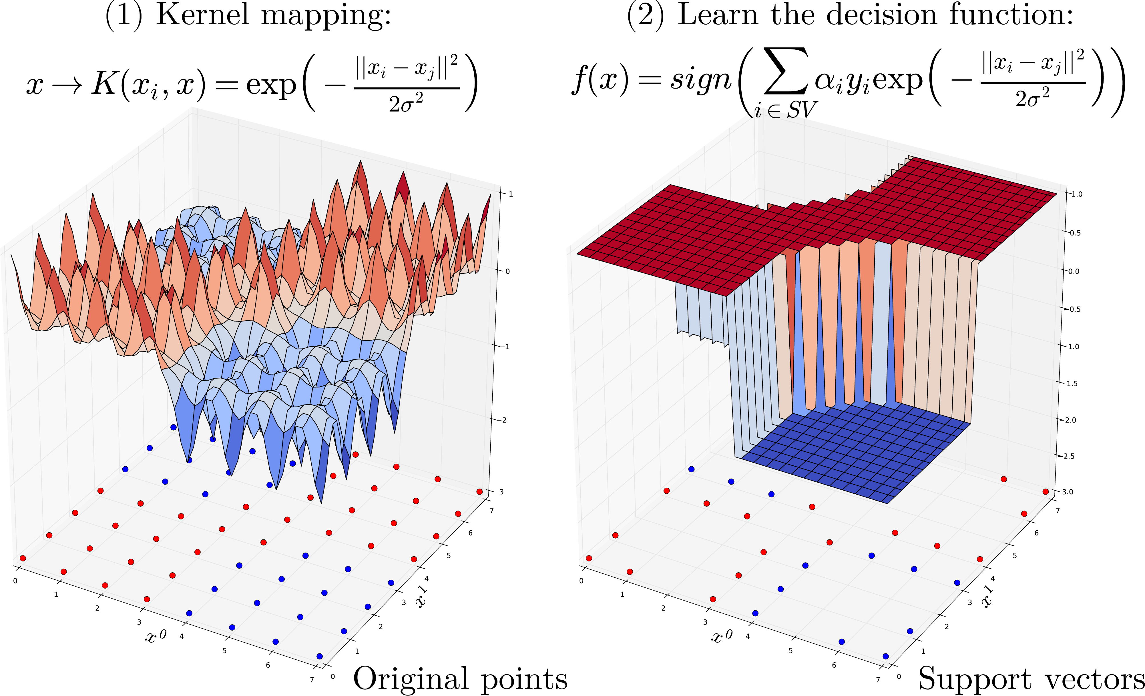
Gaussian kernel (RBF, Radial Basis Function):

One of the most commonly used kernel is the Radial Basis Function (RBF) Kernel. For a pair of points \(x_i, x_j\) the RBF kernel is defined as:

Where \(\sigma\) (or \(\gamma\)) defines the kernel width parameter. Basically, we consider a Gaussian function centered on each training sample \(x_i\). it has a ready interpretation as a similarity measure as it decreases with squared Euclidean distance between the two feature vectors.

Non linear SVM also exists for regression problems.

dataset

X, y = datasets.load_breast_cancer(return_X_y=True)
X_train, X_test, y_train, y_test = \
    train_test_split(X, y, test_size=0.5, stratify=y, random_state=42)

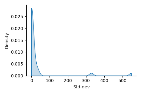
Preprocessing: unequal variance of input features, requires scaling for svm.

ax = sns.displot(x=X_train.std(axis=0), kind="kde", bw_adjust=.2, cut=0,
                 fill=True, height=3, aspect=1.5,)
_ = ax.set_xlabels("Std-dev").tight_layout()

scaler = StandardScaler()
X_train = scaler.fit_transform(X_train)
X_test = scaler.transform(X_test)

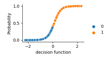
Fit-predict Probalility is a logistic of the decision_function

svm = SVC(kernel='rbf', probability=True).fit(X_train, y_train)
y_pred = svm.predict(X_test)
y_score = svm.decision_function(X_test)
y_prob = svm.predict_proba(X_test)[:, 1]

ax = sns.relplot(x=y_score, y=y_prob, hue=y_pred, height=2, aspect=1.5)
_ = ax.set_axis_labels("decision function", "Probability").tight_layout()

print("bAcc: %.2f, AUC: %.2f (AUC with proba: %.2f)" % (
      metrics.balanced_accuracy_score(y_true=y_test, y_pred=y_pred),
      metrics.roc_auc_score(y_true=y_test, y_score=y_score),
      metrics.roc_auc_score(y_true=y_test, y_score=y_prob)))

# Usefull internals: indices of support vectors within original X
np.all(X_train[svm.support_, :] == svm.support_vectors_)

Out:

bAcc: 0.96, AUC: 0.99 (AUC with proba: 0.99)

True

Random forest

Decision tree

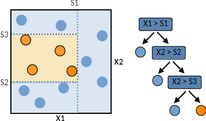
A tree can be “learned” by splitting the training dataset into subsets based on an features value test. Each internal node represents a “test” on an feature resulting on the split of the current sample. At each step the algorithm selects the feature and a cutoff value that maximises a given metric. Different metrics exist for regression tree (target is continuous) or classification tree (the target is qualitative). This process is repeated on each derived subset in a recursive manner called recursive partitioning. The recursion is completed when the subset at a node has all the same value of the target variable, or when splitting no longer adds value to the predictions. This general principle is implemented by many recursive partitioning tree algorithms.

Decision trees are simple to understand and interpret however they tend to overfit the data. However decision trees tend to overfit the training set. Leo Breiman propose random forest to deal with this issue.

A single decision tree is usually overfits the data it is learning from because it learn from only one pathway of decisions. Predictions from a single decision tree usually don’t make accurate predictions on new data.

Forest

A random forest is a meta estimator that fits a number of decision tree learners on various sub-samples of the dataset and use averaging to improve the predictive accuracy and control over-fitting. Random forest models reduce the risk of overfitting by introducing randomness by:

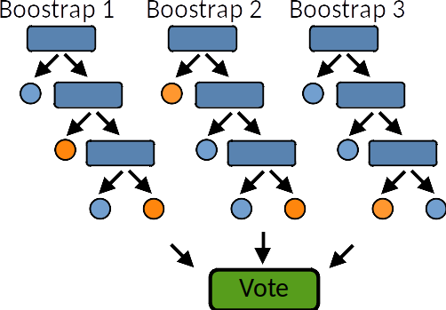
• building multiple trees (n_estimators)

• drawing observations with replacement (i.e., a bootstrapped sample)

• splitting nodes on the best split among a random subset of the features selected at every node

from sklearn.ensemble import RandomForestClassifier

forest = RandomForestClassifier(n_estimators = 100)
forest.fit(X_train, y_train)

y_pred = forest.predict(X_test)
y_prob = forest.predict_proba(X_test)[:, 1]

print("bAcc: %.2f, AUC: %.2f " % (
      metrics.balanced_accuracy_score(y_true=y_test, y_pred=y_pred),
      metrics.roc_auc_score(y_true=y_test, y_score=y_prob)))

Out:

bAcc: 0.93, AUC: 0.99

Extra Trees (Low Variance)

Extra Trees is like Random Forest, in that it builds multiple trees and splits nodes using random subsets of features, but with two key differences: it does not bootstrap observations (meaning it samples without replacement), and nodes are split on random splits, not best splits. So, in summary, ExtraTrees: builds multiple trees with bootstrap = False by default, which means it samples without replacement nodes are split based on random splits among a random subset of the features selected at every node In Extra Trees, randomness doesn’t come from bootstrapping of data, but rather comes from the random splits of all observations. ExtraTrees is named for (Extremely Randomized Trees).

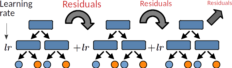
Gradient boosting

Gradient boosting is a meta estimator that fits a sequence of weak learners. Each learner aims to reduce the residuals (errors) produced by the previous learner. The two main hyper-parameters are:

• The learning rate (lr) controls over-fitting: decreasing the lr limits the capacity of a learner to overfit the residuals, ie, it slows down the learning speed and thus increases the regularisation.

• The sub-sampling fraction controls the fraction of samples to be used for fitting the learners. Values smaller than 1 leads to Stochastic Gradient Boosting. It thus controls for over-fitting reducing variance and incresing bias.

from sklearn.ensemble import GradientBoostingClassifier

gb = GradientBoostingClassifier(n_estimators=100, learning_rate=0.1,
                                subsample=0.5, random_state=0)
gb.fit(X_train, y_train)

y_pred = gb.predict(X_test)
y_prob = gb.predict_proba(X_test)[:, 1]

print("bAcc: %.2f, AUC: %.2f " % (
      metrics.balanced_accuracy_score(y_true=y_test, y_pred=y_pred),
      metrics.roc_auc_score(y_true=y_test, y_score=y_prob)))

Out:

bAcc: 0.94, AUC: 0.99