Time series in python¶

Two libraries:

Stationarity¶

A TS is said to be stationary if its statistical properties such as mean, variance remain constant over time.

constant mean
constant variance
an autocovariance that does not depend on time.

what is making a TS non-stationary. There are 2 major reasons behind non-stationaruty of a TS:

Trend – varying mean over time. For eg, in this case we saw that on average, the number of passengers was growing over time.
Seasonality – variations at specific time-frames. eg people might have a tendency to buy cars in a particular month because of pay increment or festivals.

Pandas time series data structure¶

A Series is similar to a list or an array in Python. It represents a series of values (numeric or otherwise) such as a column of data. It provides additional functionality, methods, and operators, which make it a more powerful version of a list.

%matplotlib inline

import numpy as np
import pandas as pd
import matplotlib.pyplot as plt
import seaborn as sns

# Create a Series from a list
ser = pd.Series([1, 3])
print(ser)

# String as index
prices = {'apple': 4.99,
         'banana': 1.99,
         'orange': 3.99}
ser = pd.Series(prices)
print(ser)

x = pd.Series(np.arange(1,3), index=[x for x in 'ab'])
print(x)
print(x['b'])

0    1
1    3
dtype: int64
apple     4.99
banana    1.99
orange    3.99
dtype: float64
a    1
b    2
dtype: int64
2

Time series analysis of Google trends¶

source: https://www.datacamp.com/community/tutorials/time-series-analysis-tutorial

Get Google Trends data of keywords such as ‘diet’ and ‘gym’ and see how they vary over time while learning about trends and seasonality in time series data.

In the Facebook Live code along session on the 4th of January, we checked out Google trends data of keywords ‘diet’, ‘gym’ and ‘finance’ to see how they vary over time. We asked ourselves if there could be more searches for these terms in January when we’re all trying to turn over a new leaf?

In this tutorial, you’ll go through the code that we put together during the session step by step. You’re not going to do much mathematics but you are going to do the following:

Read data
Recode data
Exploratory Data Analysis

Read data¶

try:
    url = "https://raw.githubusercontent.com/datacamp/datacamp_facebook_live_ny_resolution/master/datasets/multiTimeline.csv"
    df = pd.read_csv(url, skiprows=2)
except:
    df = pd.read_csv("../datasets/multiTimeline.csv", skiprows=2)

print(df.head())

# Rename columns
df.columns = ['month', 'diet', 'gym', 'finance']

# Describe
print(df.describe())

     Month  diet: (Worldwide)  gym: (Worldwide)  finance: (Worldwide)
0  2004-01                100                31                    48
1  2004-02                 75                26                    49
2  2004-03                 67                24                    47
3  2004-04                 70                22                    48
4  2004-05                 72                22                    43
             diet         gym     finance
count  168.000000  168.000000  168.000000
mean    49.642857   34.690476   47.148810
std      8.033080    8.134316    4.972547
min     34.000000   22.000000   38.000000
25%     44.000000   28.000000   44.000000
50%     48.500000   32.500000   46.000000
75%     53.000000   41.000000   50.000000
max    100.000000   58.000000   73.000000

Recode data¶

Next, you’ll turn the ‘month’ column into a DateTime data type and make it the index of the DataFrame.

Note that you do this because you saw in the result of the .info() method that the ‘Month’ column was actually an of data type object. Now, that generic data type encapsulates everything from strings to integers, etc. That’s not exactly what you want when you want to be looking at time series data. That’s why you’ll use .to_datetime() to convert the ‘month’ column in your DataFrame to a DateTime.

Be careful! Make sure to include the inplace argument when you’re setting the index of the DataFrame df so that you actually alter the original index and set it to the ‘month’ column.

df.month = pd.to_datetime(df.month)
df.set_index('month', inplace=True)

print(df.head())

            diet  gym  finance
month
2004-01-01   100   31       48
2004-02-01    75   26       49
2004-03-01    67   24       47
2004-04-01    70   22       48
2004-05-01    72   22       43

Exploratory data analysis¶

You can use a built-in pandas visualization method .plot() to plot your data as 3 line plots on a single figure (one for each column, namely, ‘diet’, ‘gym’, and ‘finance’).

df.plot()
plt.xlabel('Year');

# change figure parameters
# df.plot(figsize=(20,10), linewidth=5, fontsize=20)

# Plot single column
# df[['diet']].plot(figsize=(20,10), linewidth=5, fontsize=20)
# plt.xlabel('Year', fontsize=20);

Note that this data is relative. As you can read on Google trends:

Numbers represent search interest relative to the highest point on the chart for the given region and time. A value of 100 is the peak popularity for the term. A value of 50 means that the term is half as popular. Likewise a score of 0 means the term was less than 1% as popular as the peak.

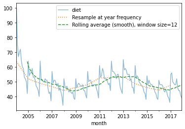
Resampling, smoothing, windowing, rolling average: trends¶

Rolling average, for each time point, take the average of the points on either side of it. Note that the number of points is specified by a window size.

Remove Seasonality with pandas Series.

See: http://pandas.pydata.org/pandas-docs/stable/timeseries.html A: ‘year end frequency’ year frequency

diet = df['diet']

diet_resamp_yr = diet.resample('A').mean()
diet_roll_yr = diet.rolling(12).mean()

ax = diet.plot(alpha=0.5, style='-') # store axis (ax) for latter plots
diet_resamp_yr.plot(style=':', label='Resample at year frequency', ax=ax)
diet_roll_yr.plot(style='--', label='Rolling average (smooth), window size=12', ax=ax)
ax.legend()

<matplotlib.legend.Legend at 0x7f670db34a10>

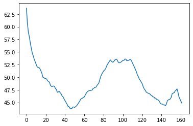
Rolling average (smoothing) with Numpy

x = np.asarray(df[['diet']])
win = 12
win_half = int(win / 2)
# print([((idx-win_half), (idx+win_half)) for idx in np.arange(win_half, len(x))])

diet_smooth = np.array([x[(idx-win_half):(idx+win_half)].mean() for idx in np.arange(win_half, len(x))])
plt.plot(diet_smooth)

[<matplotlib.lines.Line2D at 0x7f670cbbb1d0>]

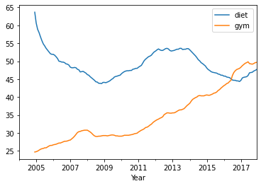
Trends Plot Diet and Gym

Build a new DataFrame which is the concatenation diet and gym smoothed data

gym = df['gym']

df_avg = pd.concat([diet.rolling(12).mean(), gym.rolling(12).mean()], axis=1)
df_avg.plot()
plt.xlabel('Year')

Text(0.5, 0, 'Year')

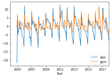
Detrending

df_dtrend = df[["diet", "gym"]] - df_avg
df_dtrend.plot()
plt.xlabel('Year')

Text(0.5, 0, 'Year')

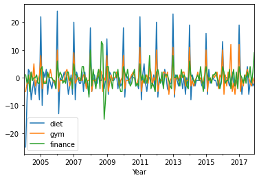
First-order differencing: seasonal patterns¶

# diff = original - shiftted data
# (exclude first term for some implementation details)
assert np.all((diet.diff() == diet - diet.shift())[1:])

df.diff().plot()
plt.xlabel('Year')

Text(0.5, 0, 'Year')

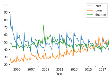
Periodicity and correlation¶

df.plot()
plt.xlabel('Year');
print(df.corr())

             diet       gym   finance
diet     1.000000 -0.100764 -0.034639
gym     -0.100764  1.000000 -0.284279
finance -0.034639 -0.284279  1.000000

Plot correlation matrix

print(df.corr())

             diet       gym   finance
diet     1.000000 -0.100764 -0.034639
gym     -0.100764  1.000000 -0.284279
finance -0.034639 -0.284279  1.000000

‘diet’ and ‘gym’ are negatively correlated! Remember that you have a seasonal and a trend component. From the correlation coefficient, ‘diet’ and ‘gym’ are negatively correlated:

trends components are negatively correlated.
seasonal components would positively correlated and their

The actual correlation coefficient is actually capturing both of those.

Seasonal correlation: correlation of the first-order differences of these time series

df.diff().plot()
plt.xlabel('Year');

print(df.diff().corr())

             diet       gym   finance
diet     1.000000  0.758707  0.373828
gym      0.758707  1.000000  0.301111
finance  0.373828  0.301111  1.000000

Plot correlation matrix

print(df.diff().corr())

             diet       gym   finance
diet     1.000000  0.758707  0.373828
gym      0.758707  1.000000  0.301111
finance  0.373828  0.301111  1.000000

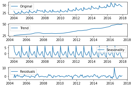
Decomposing time serie in trend, seasonality and residuals

from statsmodels.tsa.seasonal import seasonal_decompose

x = gym

x = x.astype(float) # force float
decomposition = seasonal_decompose(x)
trend = decomposition.trend
seasonal = decomposition.seasonal
residual = decomposition.resid

plt.subplot(411)
plt.plot(x, label='Original')
plt.legend(loc='best')
plt.subplot(412)
plt.plot(trend, label='Trend')
plt.legend(loc='best')
plt.subplot(413)
plt.plot(seasonal,label='Seasonality')
plt.legend(loc='best')
plt.subplot(414)
plt.plot(residual, label='Residuals')
plt.legend(loc='best')
plt.tight_layout()

Autocorrelation¶

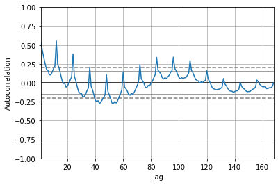
A time series is periodic if it repeats itself at equally spaced intervals, say, every 12 months. Autocorrelation Function (ACF): It is a measure of the correlation between the TS with a lagged version of itself. For instance at lag 5, ACF would compare series at time instant t1…t2 with series at instant t1-5…t2-5 (t1-5 and t2 being end points).

Plot

# from pandas.plotting import autocorrelation_plot
from pandas.plotting import autocorrelation_plot

x = df["diet"].astype(float)
autocorrelation_plot(x)

<AxesSubplot:xlabel='Lag', ylabel='Autocorrelation'>

Compute Autocorrelation Function (ACF)

from statsmodels.tsa.stattools import acf

x_diff = x.diff().dropna() # first item is NA
lag_acf = acf(x_diff, nlags=36, fft=True)
plt.plot(lag_acf)
plt.title('Autocorrelation Function')

Text(0.5, 1.0, 'Autocorrelation Function')

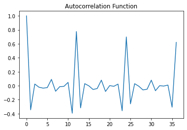
ACF peaks every 12 months: Time series is correlated with itself shifted by 12 months.

Time series forecasting with Python using Autoregressive Moving Average (ARMA) models¶

Source:

ARMA models are often used to forecast a time series. These models combine autoregressive and moving average models. In moving average models, we assume that a variable is the sum of the mean of the time series and a linear combination of noise components.

The autoregressive and moving average models can have different orders. In general, we can define an ARMA model with p autoregressive terms and q moving average terms as follows:

\[x_t = \sum_i^p a_i x_{t-i} +\sum_i^q b_i \varepsilon_{t-i} + \varepsilon_t\]

Choosing p and q¶

Plot the partial autocorrelation functions for an estimate of p, and likewise using the autocorrelation functions for an estimate of q.

Partial Autocorrelation Function (PACF): This measures the correlation between the TS with a lagged version of itself but after eliminating the variations already explained by the intervening comparisons. Eg at lag 5, it will check the correlation but remove the effects already explained by lags 1 to 4.

from statsmodels.tsa.stattools import acf, pacf

x = df["gym"].astype(float)

x_diff = x.diff().dropna() # first item is NA
# ACF and PACF plots:

lag_acf = acf(x_diff, nlags=20, fft=True)
lag_pacf = pacf(x_diff, nlags=20, method='ols')

#Plot ACF:
plt.subplot(121)
plt.plot(lag_acf)
plt.axhline(y=0,linestyle='--',color='gray')
plt.axhline(y=-1.96/np.sqrt(len(x_diff)),linestyle='--',color='gray')
plt.axhline(y=1.96/np.sqrt(len(x_diff)),linestyle='--',color='gray')
plt.title('Autocorrelation Function  (q=1)')

#Plot PACF:
plt.subplot(122)
plt.plot(lag_pacf)
plt.axhline(y=0,linestyle='--',color='gray')
plt.axhline(y=-1.96/np.sqrt(len(x_diff)),linestyle='--',color='gray')
plt.axhline(y=1.96/np.sqrt(len(x_diff)),linestyle='--',color='gray')
plt.title('Partial Autocorrelation Function (p=1)')
plt.tight_layout()

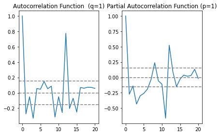
In this plot, the two dotted lines on either sides of 0 are the confidence interevals. These can be used to determine the p and q values as:

p: The lag value where the PACF chart crosses the upper confidence interval for the first time, in this case p=1.
q: The lag value where the ACF chart crosses the upper confidence interval for the first time, in this case q=1.

Fit ARMA model with statsmodels¶

Define the model by calling ARMA() and passing in the p and q parameters.
The model is prepared on the training data by calling the fit() function.
Predictions can be made by calling the predict() function and specifying the index of the time or times to be predicted.

from statsmodels.tsa.arima_model import ARMA
# from statsmodels.tsa.arima.model import ARIMA

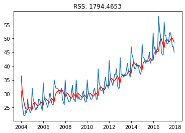
model = ARMA(x, order=(1, 1)).fit() # fit model

print(model.summary())
plt.plot(x)
plt.plot(model.predict(), color='red')
plt.title('RSS: %.4f'% sum((model.fittedvalues-x)**2))

/home/ed203246/anaconda3/lib/python3.7/site-packages/statsmodels/tsa/arima_model.py:472: FutureWarning:
statsmodels.tsa.arima_model.ARMA and statsmodels.tsa.arima_model.ARIMA have
been deprecated in favor of statsmodels.tsa.arima.model.ARIMA (note the .
between arima and model) and
statsmodels.tsa.SARIMAX. These will be removed after the 0.12 release.

statsmodels.tsa.arima.model.ARIMA makes use of the statespace framework and
is both well tested and maintained.

To silence this warning and continue using ARMA and ARIMA until they are
removed, use:

import warnings
warnings.filterwarnings('ignore', 'statsmodels.tsa.arima_model.ARMA',
                        FutureWarning)
warnings.filterwarnings('ignore', 'statsmodels.tsa.arima_model.ARIMA',
                        FutureWarning)

  warnings.warn(ARIMA_DEPRECATION_WARN, FutureWarning)
/home/ed203246/anaconda3/lib/python3.7/site-packages/statsmodels/tsa/base/tsa_model.py:527: ValueWarning: No frequency information was provided, so inferred frequency MS will be used.
  % freq, ValueWarning)

                              ARMA Model Results
==============================================================================
Dep. Variable:                    gym   No. Observations:                  168
Model:                     ARMA(1, 1)   Log Likelihood                -436.852
Method:                       css-mle   S.D. of innovations              3.229
Date:                Fri, 04 Dec 2020   AIC                            881.704
Time:                        13:05:20   BIC                            894.200
Sample:                    01-01-2004   HQIC                           886.776
                         - 12-01-2017
==============================================================================
                 coef    std err          z      P>|z|      [0.025      0.975]
------------------------------------------------------------------------------
const         36.4315      8.827      4.127      0.000      19.131      53.732
ar.L1.gym      0.9967      0.005    220.566      0.000       0.988       1.006
ma.L1.gym     -0.7494      0.054    -13.931      0.000      -0.855      -0.644
                                    Roots
=============================================================================
                  Real          Imaginary           Modulus         Frequency
-----------------------------------------------------------------------------
AR.1            1.0033           +0.0000j            1.0033            0.0000
MA.1            1.3344           +0.0000j            1.3344            0.0000
-----------------------------------------------------------------------------

Text(0.5, 1.0, 'RSS: 1794.4653')