Ensemble learning: bagging, boosting and stacking
These methods are Ensemble learning techniques. These models are machine learning paradigms where multiple models (often called “weak learners”) are trained to solve the same problem and combined to get better results. The main hypothesis is that when weak models are correctly combined we can obtain more accurate and/or robust models.
Single weak learner
In machine learning, no matter if we are facing a classification or a regression problem, the choice of the model is extremely important to have any chance to obtain good results. This choice can depend on many variables of the problem: quantity of data, dimensionality of the space, distribution hypothesis…
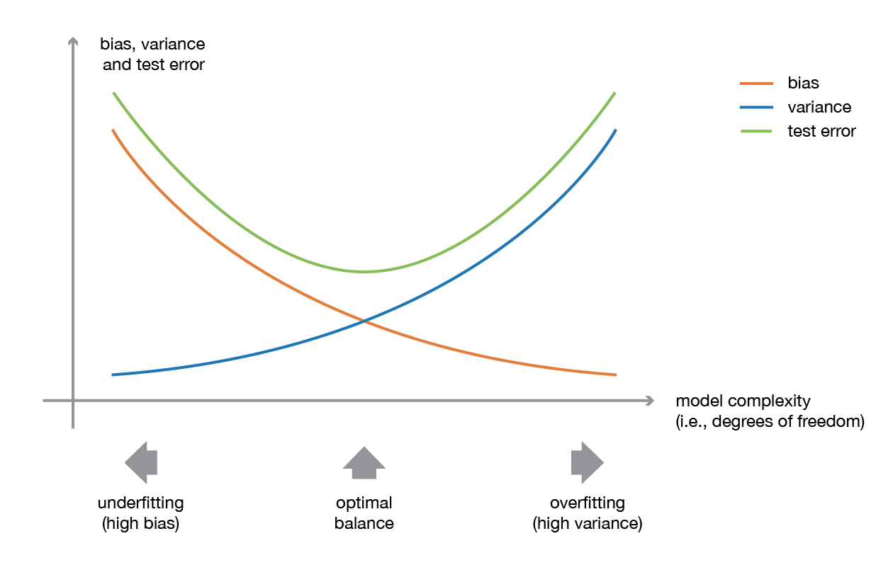
A low bias and a low variance, although they most often vary in opposite directions, are the two most fundamental features expected for a model. Indeed, to be able to “solve” a problem, we want our model to have enough degrees of freedom to resolve the underlying complexity of the data we are working with, but we also want it to have not too much degrees of freedom to avoid high variance and be more robust. This is the well known bias-variance tradeoff.
towardsdatascience blog
Illustration of the bias-variance tradeoff.
In ensemble learning theory, we call weak learners (or base models) models that can be used as building blocks for designing more complex models by combining several of them. Most of the time, these basics models perform not so well by themselves either because they have a high bias (low degree of freedom models, for example) or because they have too much variance to be robust (high degree of freedom models, for example). Then, the idea of ensemble methods is to combining several of them together in order to create a strong learner (or ensemble model) that achieves better performances.
Usually, ensemble models are used in order to :
decrease the variance for bagging (Bootstrap Aggregating) technique
reduce bias for the boosting technique
improving the predictive force for stacking technique.
To understand these techniques, first, we will explore what is boostrapping and its different hypothesis.
Bagging
In parallel methods we fit the different considered learners independently from each others and, so, it is possible to train them concurrently. The most famous such approach is “bagging” (standing for “bootstrap aggregating”) that aims at producing an ensemble model that is more robust than the individual models composing it.
When training a model, no matter if we are dealing with a classification or a regression problem, we obtain a function that takes an input, returns an output and that is defined with respect to the training dataset.
The idea of bagging is then simple: we want to fit several independent models and “average” their predictions in order to obtain a model with a lower variance. However, we can’t, in practice, fit fully independent models because it would require too much data. So, we rely on the good “approximate properties” of bootstrap samples (representativity and independence) to fit models that are almost independent.
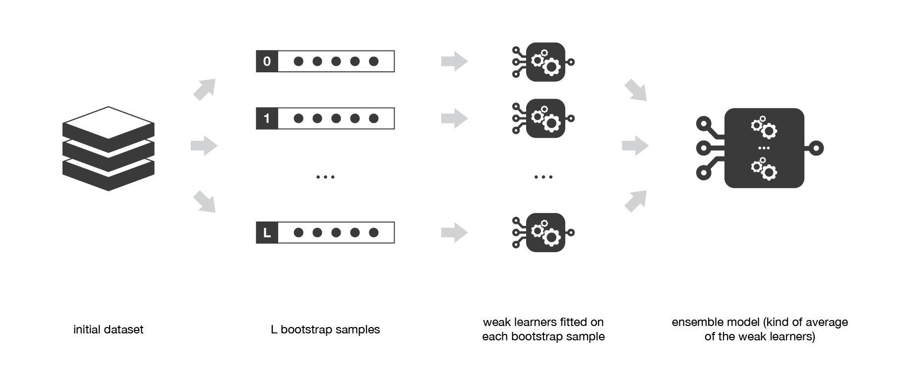
First, we create multiple bootstrap samples so that each new bootstrap sample will act as another (almost) independent dataset drawn from true distribution. Then, we can fit a weak learner for each of these samples and finally aggregate them such that we kind of “average” their outputs and, so, obtain an ensemble model with less variance that its components. Roughly speaking, as the bootstrap samples are approximatively independent and identically distributed (i.i.d.), so are the learned base models. Then, “averaging” weak learners outputs do not change the expected answer but reduce its variance.
So, assuming that we have L bootstrap samples (approximations of L independent datasets) of size B denoted

Medium Science Blog
Each {….} is a bootstrap sample of B observation
we can fit L almost independent weak learners (one on each dataset)

Medium Science Blog
and then aggregate them into some kind of averaging process in order to get an ensemble model with a lower variance. For example, we can define our strong model such that

Medium Science Blog
There are several possible ways to aggregate the multiple models fitted in parallel. - For a regression problem, the outputs of individual models can literally be averaged to obtain the output of the ensemble model. - For classification problem the class outputted by each model can be seen as a vote and the class that receives the majority of the votes is returned by the ensemble model (this is called hard-voting). Still for a classification problem, we can also consider the probabilities of each classes returned by all the models, average these probabilities and keep the class with the highest average probability (this is called soft-voting). –> Averages or votes can either be simple or weighted if any relevant weights can be used.
Finally, we can mention that one of the big advantages of bagging is that it can be parallelised. As the different models are fitted independently from each others, intensive parallelisation techniques can be used if required.
Medium Science Blog
Bagging consists in fitting several base models on different bootstrap samples and build an ensemble model that “average” the results of these weak learners.
Question : - Can you name an algorithms based on Bagging technique , Hint : leaf
###### Examples
Here, we are trying some example of stacking
Bagged Decision Trees for Classification
import pandas
from sklearn import model_selection
from sklearn.ensemble import BaggingClassifier
from sklearn.tree import DecisionTreeClassifier


names = ['preg', 'plas', 'pres', 'skin', 'test', 'mass', 'pedi', 'age', 'class']
dataframe = pandas.read_csv("https://raw.githubusercontent.com/jbrownlee/Datasets/master/pima-indians-diabetes.data.csv",names=names)

array = dataframe.values
x = array[:,0:8]
y = array[:,8]
max_features = 3

kfold = model_selection.KFold(n_splits=10, random_state=2020)
rf = DecisionTreeClassifier(max_features=max_features)
num_trees = 100

model = BaggingClassifier(base_estimator=rf, n_estimators=num_trees, random_state=2020)
results = model_selection.cross_val_score(model, x, y, cv=kfold)
print("Accuracy: %0.2f (+/- %0.2f)" % (results.mean(), results.std()))
Random Forest Classification
import pandas
from sklearn import model_selection
from sklearn.ensemble import RandomForestClassifier

names = ['preg', 'plas', 'pres', 'skin', 'test', 'mass', 'pedi', 'age', 'class']
dataframe = pandas.read_csv("https://raw.githubusercontent.com/jbrownlee/Datasets/master/pima-indians-diabetes.data.csv",names=names)

array = dataframe.values
x = array[:,0:8]
y = array[:,8]

kfold = model_selection.KFold(n_splits=10, random_state=2020)
rf = DecisionTreeClassifier()
num_trees = 100
max_features = 3

kfold = model_selection.KFold(n_splits=10, random_state=2020)
model = RandomForestClassifier(n_estimators=num_trees, max_features=max_features)
results = model_selection.cross_val_score(model, x, y, cv=kfold)
print("Accuracy: %0.2f (+/- %0.2f)" % (results.mean(), results.std()))
Both of these algorithms will print, Accuracy: 0.77 (+/- 0.07). They are equivalent.
Boosting
In sequential methods the different combined weak models are no longer fitted independently from each others. The idea is to fit models iteratively such that the training of model at a given step depends on the models fitted at the previous steps. “Boosting” is the most famous of these approaches and it produces an ensemble model that is in general less biased than the weak learners that compose it.
Boosting methods work in the same spirit as bagging methods: we build a family of models that are aggregated to obtain a strong learner that performs better.
However, unlike bagging that mainly aims at reducing variance, boosting is a technique that consists in fitting sequentially multiple weak learners in a very adaptative way: each model in the sequence is fitted giving more importance to observations in the dataset that were badly handled by the previous models in the sequence. Intuitively, each new model focus its efforts on the most difficult observations to fit up to now, so that we obtain, at the end of the process, a strong learner with lower bias (even if we can notice that boosting can also have the effect of reducing variance).
–> Boosting, like bagging, can be used for regression as well as for classification problems.
Being mainly focused at reducing bias, the base models that are often considered for boosting are* *models with low variance but high bias. For example, if we want to usetreesas our base models, we will choosemost of the time shallow decision trees with only a few depths.**
Another important reason that motivates the use of low variance but high bias models as weak learners for boosting is that these models are in general less computationally expensive to fit (few degrees of freedom when parametrised). Indeed, as computations to fit the different models can’t be done in parallel (unlike bagging), it could become too expensive to fit sequentially several complex models.
Once the weak learners have been chosen, we still need to define how they will be sequentially fitted and how they will be aggregated. We will discuss these questions in the two following subsections, describing more especially two important boosting algorithms: adaboost and gradient boosting.
In a nutshell, these two meta-algorithms differ on how they create and aggregate the weak learners during the sequential process. Adaptive boosting updates the weights attached to each of the training dataset observations whereas gradient boosting updates the value of these observations. This main difference comes from the way both methods try to solve the optimisation problem of finding the best model that can be written as a weighted sum of weak learners.
Medium Science Blog
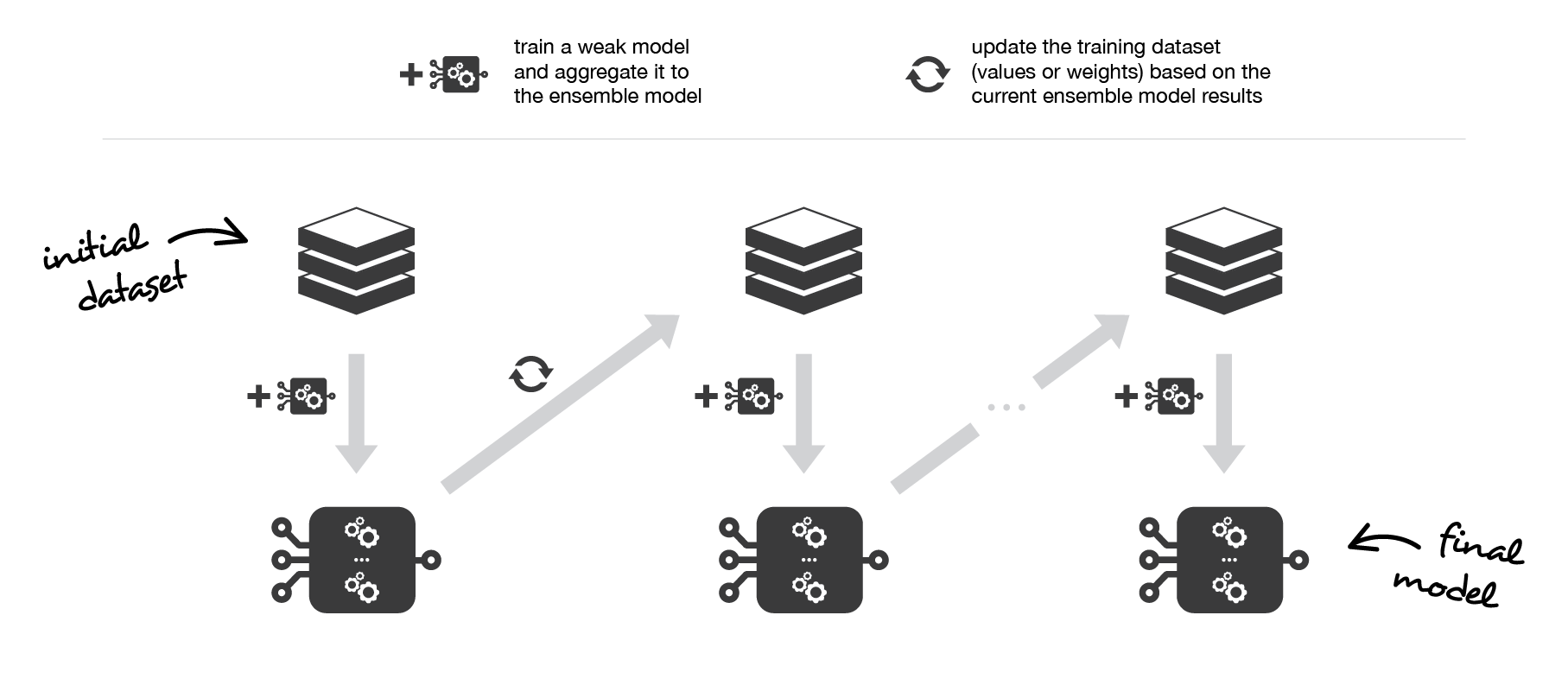
Boosting consists in, iteratively, fitting a weak learner, aggregate it to the ensemble model and “update” the training dataset to better take into account the strengths and weakness of the current ensemble model when fitting the next base model.
1/ Adaptative boosting
In adaptative boosting (often called “adaboost”), we try to define our ensemble model as a weighted sum of L weak learners

Medium Science Blog
Finding the best ensemble model with this form is a difficult optimisation problem. Then, instead of trying to solve it in one single shot (finding all the coefficients and weak learners that give the best overall additive model), we make use of an iterative optimisation process that is much more tractable, even if it can lead to a sub-optimal solution. More especially, we add the weak learners one by one, looking at each iteration for the best possible pair (coefficient, weak learner) to add to the current ensemble model. In other words, we define recurrently the (s_l)’s such that

towardsdatascience Blog
where c_l and w_l are chosen such that s_l is the model that fit the best the training data and, so, that is the best possible improvement over s_(l-1). We can then denote

towardsdatascience Blog
where E(.) is the fitting error of the given model and e(.,.) is the loss/error function. Thus, instead of optimising “globally” over all the L models in the sum, we approximate the optimum by optimising “locally” building and adding the weak learners to the strong model one by one.
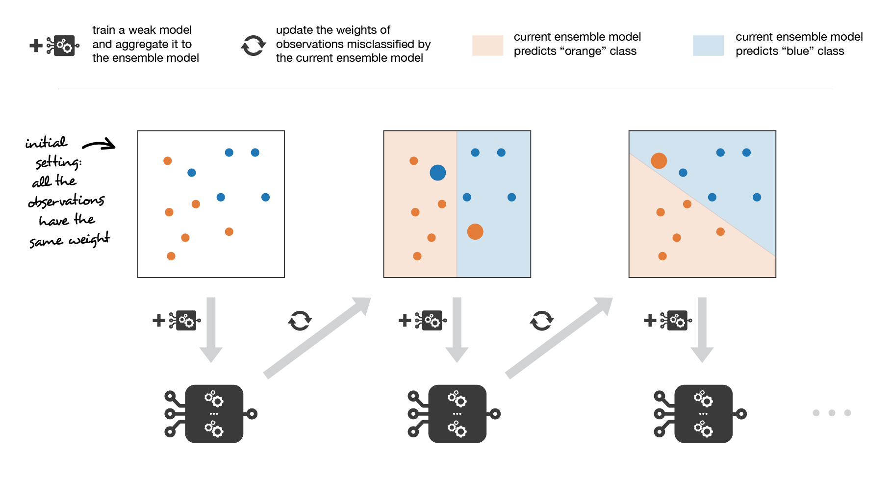
More especially, when considering a binary classification, we can show that the adaboost algorithm can be re-written into a process that proceeds as follow. First, it updates the observations weights in the dataset and train a new weak learner with a special focus given to the observations misclassified by the current ensemble model. Second, it adds the weak learner to the weighted sum according to an update coefficient that expresse the performances of this weak model: the better a weak learner performs, the more it contributes to the strong learner.
So, assume that we are facing a binary classification problem, with N observations in our dataset and we want to use adaboost algorithm with a given family of weak models. At the very beginning of the algorithm (first model of the sequence), all the observations have the same weights 1/N. Then, we repeat L times (for the L learners in the sequence) the following steps:
fit the best possible weak model with the current observations weights
compute the value of the update coefficient that is some kind of scalar evaluation metric of the weak learner that indicates how much this weak learner should be taken into account into the ensemble model
update the strong learner by adding the new weak learner multiplied by its update coefficient
compute new observations weights that expresse which observations we would like to focus on at the next iteration (weights of observations wrongly predicted by the aggregated model increase and weights of the correctly predicted observations decrease)
Repeating these steps, we have then build sequentially our L models and aggregate them into a simple linear combination weighted by coefficients expressing the performance of each learner.
Notice that there exists variants of the initial adaboost algorithm such that LogitBoost (classification) or L2Boost (regression) that mainly differ by their choice of loss function.
Medium Science Blog
Adaboost updates weights of the observations at each iteration. Weights of well classified observations decrease relatively to weights of misclassified observations. Models that perform better have higher weights in the final ensemble model.
2/ Gradient boosting
In gradient boosting, the ensemble model we try to build is also a weighted sum of weak learners
Medium Science Blog
Just as we mentioned for adaboost, finding the optimal model under this form is too difficult and an iterative approach is required. The main difference with adaptative boosting is in the definition of the sequential optimisation process. Indeed, gradient boosting casts the problem into a gradient descent one: at each iteration we fit a weak learner to the opposite of the gradient of the current fitting error with respect to the current ensemble model. Let’s try to clarify this last point. First, theoretical gradient descent process over the ensemble model can be written

Medium Science Blog
where E(.) is the fitting error of the given model, c_l is a coefficient corresponding to the step size and

Medium Science Blog
This entity is the opposite of the gradient of the fitting error with respect to the ensemble model at step l-1. This opposite of the gradient is a function that can, in practice, only be evaluated for observations in the training dataset (for which we know inputs and outputs): these evaluations are called pseudo-residuals attached to each observations. Moreover, even if we know for the observations the values of these pseudo-residuals, we don’t want to add to our ensemble model any kind of function: we only want to add a new instance of weak model. So, the natural thing to do is to fit a weak learner to the pseudo-residuals computed for each observation. Finally, the coefficient c_l is computed following a one dimensional optimisation process (line-search to obtain the best step size c_l).
So, assume that we want to use gradient boosting technique with a given family of weak models. At the very beginning of the algorithm (first model of the sequence), the pseudo-residuals are set equal to the observation values. Then, we repeat L times (for the L models of the sequence) the following steps:
fit the best possible weak model to pseudo-residuals (approximate the opposite of the gradient with respect to the current strong learner)
compute the value of the optimal step size that defines by how much we update the ensemble model in the direction of the new weak learner
update the ensemble model by adding the new weak learner multiplied by the step size (make a step of gradient descent)
compute new pseudo-residuals that indicate, for each observation, in which direction we would like to update next the ensemble model predictions
Repeating these steps, we have then build sequentially our L models and aggregate them following a gradient descent approach. Notice that, while adaptative boosting tries to solve at each iteration exactly the “local” optimisation problem (find the best weak learner and its coefficient to add to the strong model), gradient boosting uses instead a gradient descent approach and can more easily be adapted to large number of loss functions. Thus, gradient boosting can be considered as a generalization of adaboost to arbitrary differentiable loss functions.
Note There is an algorithm which gained huge popularity after a Kaggle’s competitions. It is XGBoost (Extreme Gradient Boosting). This is a gradient boosting algorithm which has more flexibility (varying number of terminal nodes and left weights) parameters to avoid sub-learners correlations. Having these important qualities, XGBOOST is one of the most used algorithm in data science. LIGHTGBM is a recent implementation of this algorithm. It was published by Microsoft and it gives us the same scores (if parameters are equivalents) but it runs quicker than a classic XGBOOST.
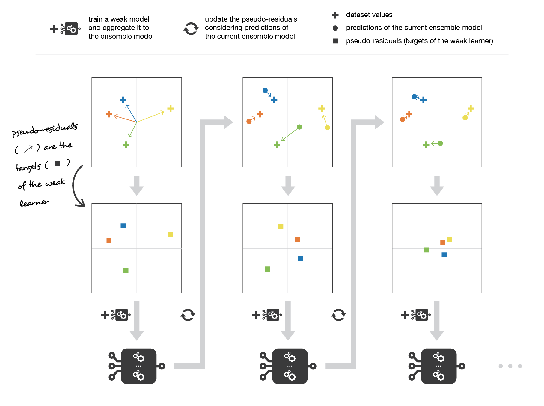
Medium Science Blog
Gradient boosting updates values of the observations at each iteration. Weak learners are trained to fit the pseudo-residuals that indicate in which direction to correct the current ensemble model predictions to lower the error.
Examples
Here, we are trying an example of Boosting and compare it to a Bagging. Both of algorithms take the same weak learners to build the macro-model
Adaboost Classifier
from sklearn.ensemble import AdaBoostClassifier
from sklearn.tree import DecisionTreeClassifier
from sklearn.datasets import load_breast_cancer
import pandas as pd
import numpy as np
from sklearn.model_selection import train_test_split
from sklearn.metrics import confusion_matrix
from sklearn.preprocessing import LabelEncoder
from sklearn.metrics import accuracy_score
from sklearn.metrics import f1_score

breast_cancer = load_breast_cancer()
x = pd.DataFrame(breast_cancer.data, columns=breast_cancer.feature_names)
y = pd.Categorical.from_codes(breast_cancer.target, breast_cancer.target_names)
# Transforming string Target to an int
encoder = LabelEncoder()
binary_encoded_y = pd.Series(encoder.fit_transform(y))

#Train Test Split
train_x, test_x, train_y, test_y = train_test_split(x, binary_encoded_y, random_state=1)
clf_boosting = AdaBoostClassifier(
    DecisionTreeClassifier(max_depth=1),
    n_estimators=200
)
clf_boosting.fit(train_x, train_y)
predictions = clf_boosting.predict(test_x)
print("For Boosting : F1 Score {}, Accuracy {}".format(round(f1_score(test_y,predictions),2),round(accuracy_score(test_y,predictions),2)))
Random Forest as a bagging classifier
from sklearn.ensemble import AdaBoostClassifier
from sklearn.tree import DecisionTreeClassifier
from sklearn.datasets import load_breast_cancer
import pandas as pd
import numpy as np
from sklearn.model_selection import train_test_split
from sklearn.metrics import confusion_matrix
from sklearn.preprocessing import LabelEncoder
from sklearn.metrics import accuracy_score
from sklearn.metrics import f1_score
from sklearn.ensemble import RandomForestClassifier

breast_cancer = load_breast_cancer()
x = pd.DataFrame(breast_cancer.data, columns=breast_cancer.feature_names)
y = pd.Categorical.from_codes(breast_cancer.target, breast_cancer.target_names)
# Transforming string Target to an int
encoder = LabelEncoder()
binary_encoded_y = pd.Series(encoder.fit_transform(y))

#Train Test Split
train_x, test_x, train_y, test_y = train_test_split(x, binary_encoded_y, random_state=1)
clf_bagging = RandomForestClassifier(n_estimators=200, max_depth=1)
clf_bagging.fit(train_x, train_y)
predictions = clf_bagging.predict(test_x)
print("For Bagging : F1 Score {}, Accuracy {}".format(round(f1_score(test_y,predictions),2),round(accuracy_score(test_y,predictions),2)))
Comparaison
Metric |
Bagging |
Boosting |
|---|---|---|
Accuracy |
0.91 |
0.97 |
F1-Score |
0.88 |
0.95 |
Overview of stacking
Stacking mainly differ from bagging and boosting on two points : - First stacking often considers heterogeneous weak learners (different learning algorithms are combined) whereas bagging and boosting consider mainly homogeneous weak learners. - Second, stacking learns to combine the base models using a meta-model whereas bagging and boosting combine weak learners following deterministic algorithms.
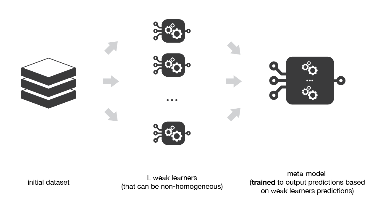
As we already mentioned, the idea of stacking is to learn several different weak learners and combine them by training a meta-model to output predictions based on the multiple predictions returned by these weak models. So, we need to define two things in order to build our stacking model: the L learners we want to fit and the meta-model that combines them.
For example, for a classification problem, we can choose as weak learners a KNN classifier, a logistic regression and a SVM, and decide to learn a neural network as meta-model. Then, the neural network will take as inputs the outputs of our three weak learners and will learn to return final predictions based on it.
So, assume that we want to fit a stacking ensemble composed of L weak learners. Then we have to follow the steps thereafter:
split the training data in two folds
choose L weak learners and fit them to data of the first fold
for each of the L weak learners, make predictions for observations in the second fold
fit the meta-model on the second fold, using predictions made by the weak learners as inputs
In the previous steps, we split the dataset in two folds because predictions on data that have been used for the training of the weak learners are not relevant for the training of the meta-model.
Medium Science Blog
Stacking consists in training a meta-model to produce outputs based on the outputs returned by some lower layer weak learners.
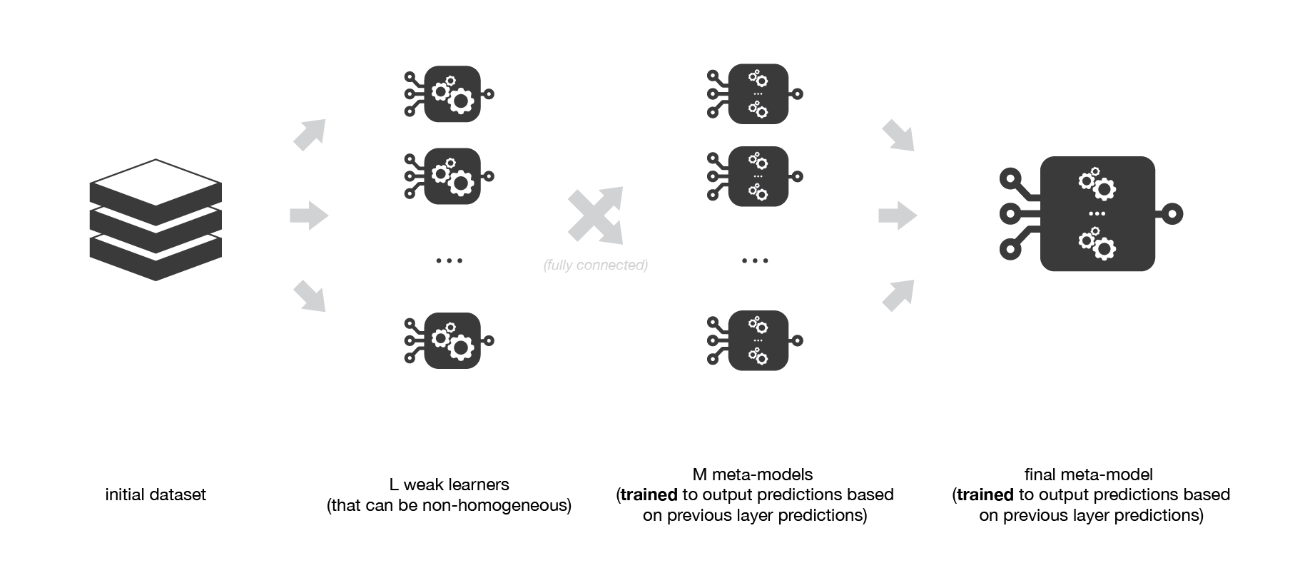
A possible extension of stacking is multi-level stacking. It consists in doing stacking with multiple layers. As an example,
Medium Science Blog
Multi-level stacking considers several layers of stacking: some meta-models are trained on outputs returned by lower layer meta-models and so on. Here we have represented a 3-layers stacking model.
Examples
Here, we are trying an example of Stacking and compare it to a Bagging & a Boosting. We note that, many other applications (datasets) would show more difference between these techniques.
from sklearn.ensemble import AdaBoostClassifier
from sklearn.tree import DecisionTreeClassifier
from sklearn.datasets import load_breast_cancer
import pandas as pd
import numpy as np
from sklearn.model_selection import train_test_split
from sklearn.metrics import confusion_matrix
from sklearn.preprocessing import LabelEncoder
from sklearn.metrics import accuracy_score
from sklearn.metrics import f1_score
from sklearn.ensemble import RandomForestClassifier
from sklearn.linear_model import LogisticRegression

breast_cancer = load_breast_cancer()
x = pd.DataFrame(breast_cancer.data, columns=breast_cancer.feature_names)
y = pd.Categorical.from_codes(breast_cancer.target, breast_cancer.target_names)

# Transforming string Target to an int
encoder = LabelEncoder()
binary_encoded_y = pd.Series(encoder.fit_transform(y))

#Train Test Split
train_x, test_x, train_y, test_y = train_test_split(x, binary_encoded_y, random_state=2020)

boosting_clf_ada_boost= AdaBoostClassifier(
    DecisionTreeClassifier(max_depth=1),
    n_estimators=3
)
bagging_clf_rf = RandomForestClassifier(n_estimators=200, max_depth=1,random_state=2020)


clf_rf = RandomForestClassifier(n_estimators=200, max_depth=1,random_state=2020)
clf_ada_boost = AdaBoostClassifier(
    DecisionTreeClassifier(max_depth=1,random_state=2020),
    n_estimators=3
)

clf_logistic_reg = LogisticRegression(solver='liblinear',random_state=2020)

#Customizing and Exception message
class NumberOfClassifierException(Exception):
    pass

#Creating a stacking class
class Stacking():

    '''
        This is a test class for stacking !
        Please fill Free to change it to fit your needs
        We suppose that at least the First N-1 Classifiers have
        a predict_proba function.
    '''

    def __init__(self,classifiers):
        if(len(classifiers) < 2):
            raise numberOfClassifierException("You must fit your classifier with 2 classifiers at least");
        else:
            self._classifiers = classifiers


    def fit(self,data_x,data_y):

        stacked_data_x = data_x.copy()
        for classfier in self._classifiers[:-1]:
            classfier.fit(data_x,data_y)
            stacked_data_x = np.column_stack((stacked_data_x,classfier.predict_proba(data_x)))


        last_classifier = self._classifiers[-1]
        last_classifier.fit(stacked_data_x,data_y)


    def predict(self,data_x):

        stacked_data_x = data_x.copy()
        for classfier in self._classifiers[:-1]:
            prob_predictions = classfier.predict_proba(data_x)
            stacked_data_x = np.column_stack((stacked_data_x,prob_predictions))

        last_classifier = self._classifiers[-1]
        return last_classifier.predict(stacked_data_x)


bagging_clf_rf.fit(train_x, train_y)
boosting_clf_ada_boost.fit(train_x, train_y)

classifers_list = [clf_rf,clf_ada_boost,clf_logistic_reg]
clf_stacking = Stacking(classifers_list)
clf_stacking.fit(train_x,train_y)

predictions_bagging = bagging_clf_rf.predict(test_x)
predictions_boosting = boosting_clf_ada_boost.predict(test_x)
predictions_stacking = clf_stacking.predict(test_x)

print("For Bagging : F1 Score {}, Accuracy {}".format(round(f1_score(test_y,predictions_bagging),2),round(accuracy_score(test_y,predictions_bagging),2)))
print("For Boosting : F1 Score {}, Accuracy {}".format(round(f1_score(test_y,predictions_boosting),2),round(accuracy_score(test_y,predictions_boosting),2)))
print("For Stacking : F1 Score {}, Accuracy {}".format(round(f1_score(test_y,predictions_stacking),2),round(accuracy_score(test_y,predictions_stacking),2)))
Comparaison
Metric |
Bagging |
Boosting |
Stacking |
|---|---|---|---|
Accuracy |
0.90 |
0.94 |
0.98 |
F1-Score |
0.88 |
0.93 |
0.98 |