Linear models for regression problems
Linear regression
Ordinary least squares
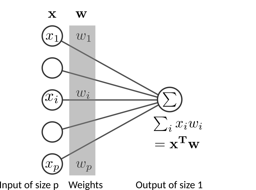
Linear regression models the output, or target variable \(y \in \mathrm{R}\) as a linear combination of the \(P\)-dimensional input \(\mathbf{x} \in \mathbb{R}^{P}\). Let \(\mathbf{X}\) be the \(N \times P\) matrix with each row an input vector (with a 1 in the first position), and similarly let \(\mathbf{y}\) be the \(N\)-dimensional vector of outputs in the training set, the linear model will predict the \(\mathbf{y}\) given \(\mathbf{x}\) using the parameter vector, or weight vector \(\mathbf{w} \in \mathbb{R}^P\) according to
where \(\boldsymbol{\varepsilon} \in \mathrm{R}^N\) are the residuals, or the errors of the prediction. The \(\mathbf{w}\) is found by minimizing an objective function, which is the loss function, \(L(\mathbf{w})\), i.e. the error measured on the data. This error is the sum of squared errors (SSE) loss.
Minimizing the SSE is the Ordinary Least Square OLS regression as objective function. which is a simple ordinary least squares (OLS) minimization whose analytic solution is:
The gradient of the loss:
Linear regression with scikit-learn
Scikit learn offer many models for supervised learning, and they all follow the same application programming interface (API), namely:
model = Estimator()
model.fit(X, y)
predictions = model.predict(X)
%matplotlib inline

import numpy as np
import pandas as pd
import matplotlib.pyplot as plt

from sklearn import datasets
import sklearn.linear_model as lm
import sklearn.metrics as metrics

np.set_printoptions(precision=2)
pd.set_option('precision', 2)
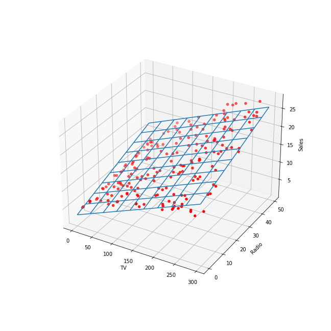
Linear regression of Advertising.csv dataset with TV and Radio
advertising as input features and Sales as target. The linear model that
minimizes the MSE is a plan (2 input features) defined as: Sales = 0.05
TV + .19 Radio + 3:
Linear regression
Overfitting
In statistics and machine learning, overfitting occurs when a statistical model describes random errors or noise instead of the underlying relationships. Overfitting generally occurs when a model is excessively complex, such as having too many parameters relative to the number of observations. A model that has been overfit will generally have poor predictive performance, as it can exaggerate minor fluctuations in the data.
A learning algorithm is trained using some set of training samples. If the learning algorithm has the capacity to overfit the training samples the performance on the training sample set will improve while the performance on unseen test sample set will decline.
The overfitting phenomenon has three main explanations: - excessively complex models, - multicollinearity, and - high dimensionality.
Model complexity
Complex learners with too many parameters relative to the number of observations may overfit the training dataset.
Multicollinearity
Predictors are highly correlated, meaning that one can be linearly predicted from the others. In this situation the coefficient estimates of the multiple regression may change erratically in response to small changes in the model or the data. Multicollinearity does not reduce the predictive power or reliability of the model as a whole, at least not within the sample data set; it only affects computations regarding individual predictors. That is, a multiple regression model with correlated predictors can indicate how well the entire bundle of predictors predicts the outcome variable, but it may not give valid results about any individual predictor, or about which predictors are redundant with respect to others. In case of perfect multicollinearity the predictor matrix is singular and therefore cannot be inverted. Under these circumstances, for a general linear model \(\mathbf{y} = \mathbf{X} \mathbf{w} + \boldsymbol{\varepsilon}\), the ordinary least-squares estimator, \(\mathbf{w}_{OLS} = (\mathbf{X}^T \mathbf{X})^{-1}\mathbf{X}^T \mathbf{y}\), does not exist.
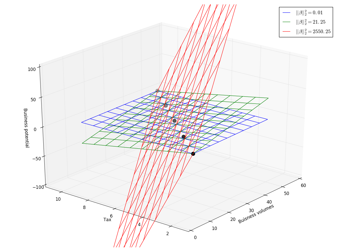
An example where correlated predictor may produce an unstable model follows: We want to predict the business potential (pb) of some companies given their business volume (bv) and the taxes (tx) they are paying. Here pb ~ 10% of bv. However, taxes = 20% of bv (tax and bv are highly collinear), therefore there is an infinite number of linear combinations of tax and bv that lead to the same prediction. Solutions with very large coefficients will produce excessively large predictions.
bv = np.array([10, 20, 30, 40, 50])             # business volume
tax  = .2 * bv                                  # Tax
bp = .1 * bv + np.array([-.1, .2, .1, -.2, .1]) # business potential

X = np.column_stack([bv, tax])
beta_star = np.array([.1, 0])  # true solution

'''
Since tax and bv are correlated, there is an infinite number of linear combinations
leading to the same prediction.
'''

# 10 times the bv then subtract it 9 times using the tax variable:
beta_medium = np.array([.1 * 10, -.1 * 9 * (1/.2)])
# 100 times the bv then subtract it 99 times using the tax variable:
beta_large = np.array([.1 * 100, -.1 * 99 * (1/.2)])

print("L2 norm of coefficients: small:%.2f, medium:%.2f, large:%.2f." %
      (np.sum(beta_star ** 2), np.sum(beta_medium ** 2), np.sum(beta_large ** 2)))

print("However all models provide the exact same predictions.")
assert np.all(np.dot(X, beta_star) == np.dot(X, beta_medium))
assert np.all(np.dot(X, beta_star) == np.dot(X, beta_large))
L2 norm of coefficients: small:0.01, medium:21.25, large:2550.25.
However all models provide the exact same predictions.
Multicollinearity between the predictors: business volumes and tax
produces unstable models with arbitrary large coefficients.
Dealing with multicollinearity:
Regularisation by e.g. \(\ell_2\) shrinkage: Introduce a bias in the solution by making \((X^T X)^{-1}\) non-singular. See \(\ell_2\) shrinkage.
Feature selection: select a small number of features. See: Isabelle Guyon and André Elisseeff An introduction to variable and feature selection The Journal of Machine Learning Research, 2003.
Feature selection: select a small number of features using \(\ell_1\) shrinkage.
Extract few independent (uncorrelated) features using e.g. principal components analysis (PCA), partial least squares regression (PLS-R) or regression methods that cut the number of predictors to a smaller set of uncorrelated components.
High dimensionality
High dimensions means a large number of input features. Linear predictor associate one parameter to each input feature, so a high-dimensional situation (\(P\), number of features, is large) with a relatively small number of samples \(N\) (so-called large \(P\) small \(N\) situation) generally lead to an overfit of the training data. Thus it is generally a bad idea to add many input features into the learner. This phenomenon is called the curse of dimensionality.
One of the most important criteria to use when choosing a learning algorithm is based on the relative size of \(P\) and \(N\).
Remenber that the “covariance” matrix \(\mathbf{X}^T\mathbf{X}\) used in the linear model is a \(P \times P\) matrix of rank \(\min(N, P)\). Thus if \(P > N\) the equation system is overparameterized and admit an infinity of solutions that might be specific to the learning dataset. See also ill-conditioned or singular matrices.
The sampling density of \(N\) samples in an \(P\)-dimensional space is proportional to \(N^{1/P}\). Thus a high-dimensional space becomes very sparse, leading to poor estimations of samples densities. To preserve a constant density, an exponential growth in the number of observations is required. 50 points in 1D, would require 2 500 points in 2D and 125 000 in 3D!
Another consequence of the sparse sampling in high dimensions is that all sample points are close to an edge of the sample. Consider \(N\) data points uniformly distributed in a \(P\)-dimensional unit ball centered at the origin. Suppose we consider a nearest-neighbor estimate at the origin. The median distance from the origin to the closest data point is given by the expression: \(d(P, N) = \left(1 - \frac{1}{2}^{1/N}\right)^{1/P}.\)
A more complicated expression exists for the mean distance to the closest point. For N = 500, P = 10 , \(d(P, N ) \approx 0.52\), more than halfway to the boundary. Hence most data points are closer to the boundary of the sample space than to any other data point. The reason that this presents a problem is that prediction is much more difficult near the edges of the training sample. One must extrapolate from neighboring sample points rather than interpolate between them. (Source: T Hastie, R Tibshirani, J Friedman.The Elements of Statistical Learning: Data Mining, Inference, and Prediction.* Second Edition, 2009.)*
Structural risk minimization provides a theoretical background of this phenomenon. (See VC dimension.)
See also bias–variance trade-off.
Regularization using penalization of coefficients
Regarding linear models, overfitting generally leads to excessively complex solutions (coefficient vectors), accounting for noise or spurious correlations within predictors. Regularization aims to alleviate this phenomenon by constraining (biasing or reducing) the capacity of the learning algorithm in order to promote simple solutions. Regularization penalizes “large” solutions forcing the coefficients to be small, i.e. to shrink them toward zeros.
The objective function \(J(\mathbf{w})\) to minimize with respect to \(\mathbf{w}\) is composed of a loss function \(L(\mathbf{w})\) for goodness-of-fit and a penalty term \(\Omega(\mathbf{w})\) (regularization to avoid overfitting). This is a trade-off where the respective contribution of the loss and the penalty terms is controlled by the regularization parameter \(\lambda\).
Therefore the loss function \(L(\mathbf{w})\) is combined with a penalty function \(\Omega(\mathbf{w})\) leading to the general form:
The respective contribution of the loss and the penalty is controlled by the regularization parameter \(\lambda\).
For regression problems the loss is the SSE given by:
Popular penalties are:
Ridge (also called \(\ell_2\)) penalty: \(\|\mathbf{w}\|_2^2\). It shrinks coefficients toward 0.
Lasso (also called \(\ell_1\)) penalty: \(\|\mathbf{w}\|_1\). It performs feature selection by setting some coefficients to 0.
ElasticNet (also called \(\ell_1\ell_2\)) penalty: \(\alpha \left(\rho~\|\mathbf{w}\|_1 + (1-\rho)~\|\mathbf{w}\|_2^2 \right)\). It performs selection of group of correlated features by setting some coefficients to 0.
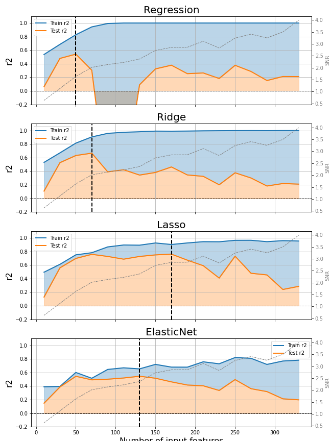
The next figure shows the predicted performance (r-squared) on train and test sets with an increasing number of input features. The number of predictive features is always 10% of the total number of input features. Therefore, the signal to noise ratio (SNR) increases by increasing the number of input features. The performances on the training set rapidly reach 100% (R2=1). However, the performance on the test set decreases with the increase of the input dimensionality. The difference between the train and test performances (blue shaded region) depicts the overfitting phenomena. Regularisation using penalties of the coefficient vector norm greatly limits the overfitting phenomena.
Multicollinearity between the predictors
With scikit-learn:
# Dataset with some correlation
X, y, coef = datasets.make_regression(n_samples=100, n_features=10, n_informative=5, random_state=0,
                                      effective_rank=3, coef=True)

lr = lm.LinearRegression().fit(X, y)

l2 = lm.Ridge(alpha=10).fit(X, y)  # lambda is alpha!

l1 = lm.Lasso(alpha=.1).fit(X, y)  # lambda is alpha !

l1l2 = lm.ElasticNet(alpha=.1, l1_ratio=.9).fit(X, y)

pd.DataFrame(np.vstack((coef, lr.coef_, l2.coef_, l1.coef_, l1l2.coef_)),
             index=['True', 'lr', 'l2', 'l1', 'l1l2'])
| 0 | 1 | 2 | 3 | 4 | 5 | 6 | 7 | 8 | 9 | |
|---|---|---|---|---|---|---|---|---|---|---|
| True | 28.49 | 0.00e+00 | 13.17 | 0.00e+00 | 48.97 | 70.44 | 39.70 | 0.00e+00 | 0.00e+00 | 0.00e+00 |
| lr | 28.49 | 3.18e-14 | 13.17 | -3.05e-14 | 48.97 | 70.44 | 39.70 | -2.48e-14 | 4.94e-14 | -2.63e-14 |
| l2 | 1.03 | 2.11e-01 | 0.93 | -3.16e-01 | 1.82 | 1.57 | 2.10 | -1.14e+00 | -8.39e-01 | -1.02e+00 |
| l1 | 0.00 | -0.00e+00 | 0.00 | -0.00e+00 | 24.40 | 25.16 | 25.36 | -0.00e+00 | -0.00e+00 | -0.00e+00 |
| l1l2 | 0.78 | 0.00e+00 | 0.51 | -0.00e+00 | 7.20 | 5.71 | 8.95 | -1.38e+00 | -0.00e+00 | -4.01e-01 |
Ridge regression (\(\ell_2\)-regularization)
Ridge regression impose a \(\ell_2\) penalty on the coefficients, i.e. it penalizes with the Euclidean norm of the coefficients while minimizing SSE. The objective function becomes:
The \(\mathbf{w}\) that minimises \(F_{Ridge}(\mathbf{w})\) can be found by the following derivation:
The solution adds a positive constant to the diagonal of \(\mathbf{X}^T\mathbf{X}\) before inversion. This makes the problem nonsingular, even if \(\mathbf{X}^T\mathbf{X}\) is not of full rank, and was the main motivation behind ridge regression.
Increasing \(\lambda\) shrinks the \(\mathbf{w}\) coefficients toward 0.
This approach penalizes the objective function by the Euclidian (:math:`ell_2`) norm of the coefficients such that solutions with large coefficients become unattractive.
The gradient of the loss:
Lasso regression (\(\ell_1\)-regularization)
Lasso regression penalizes the coefficients by the \(\ell_1\) norm. This constraint will reduce (bias) the capacity of the learning algorithm. To add such a penalty forces the coefficients to be small, i.e. it shrinks them toward zero. The objective function to minimize becomes:
This penalty forces some coefficients to be exactly zero, providing a feature selection property.
Sparsity of the \(\ell_1\) norm
Occam’s razor
Occam’s razor (also written as Ockham’s razor, and lex parsimoniae in Latin, which means law of parsimony) is a problem solving principle attributed to William of Ockham (1287-1347), who was an English Franciscan friar and scholastic philosopher and theologian. The principle can be interpreted as stating that among competing hypotheses, the one with the fewest assumptions should be selected.
Principle of parsimony
The simplest of two competing theories is to be preferred. Definition of parsimony: Economy of explanation in conformity with Occam’s razor.
Among possible models with similar loss, choose the simplest one:
Choose the model with the smallest coefficient vector, i.e. smallest \(\ell_2\) (\(\|\mathbf{w}\|_2\)) or \(\ell_1\) (\(\|\mathbf{w}\|_1\)) norm of \(\mathbf{w}\), i.e. \(\ell_2\) or \(\ell_1\) penalty. See also bias-variance tradeoff.
Choose the model that uses the smallest number of predictors. In other words, choose the model that has many predictors with zero weights. Two approaches are available to obtain this: (i) Perform a feature selection as a preprocessing prior to applying the learning algorithm, or (ii) embed the feature selection procedure within the learning process.
Sparsity-induced penalty or embedded feature selection with the \(\ell_1\) penalty
The penalty based on the \(\ell_1\) norm promotes sparsity (scattered, or not dense): it forces many coefficients to be exactly zero. This also makes the coefficient vector scattered.
The figure bellow illustrates the OLS loss under a constraint acting on the \(\ell_1\) norm of the coefficient vector. I.e., it illustrates the following optimization problem:
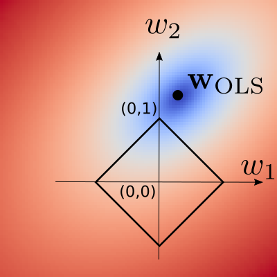
Sparsity of L1 norm
Optimization issues
Section to be completed
No more closed-form solution.
Convex but not differentiable.
Requires specific optimization algorithms, such as the fast iterative shrinkage-thresholding algorithm (FISTA): Amir Beck and Marc Teboulle, A Fast Iterative Shrinkage-Thresholding Algorithm for Linear Inverse Problems SIAM J. Imaging Sci., 2009.
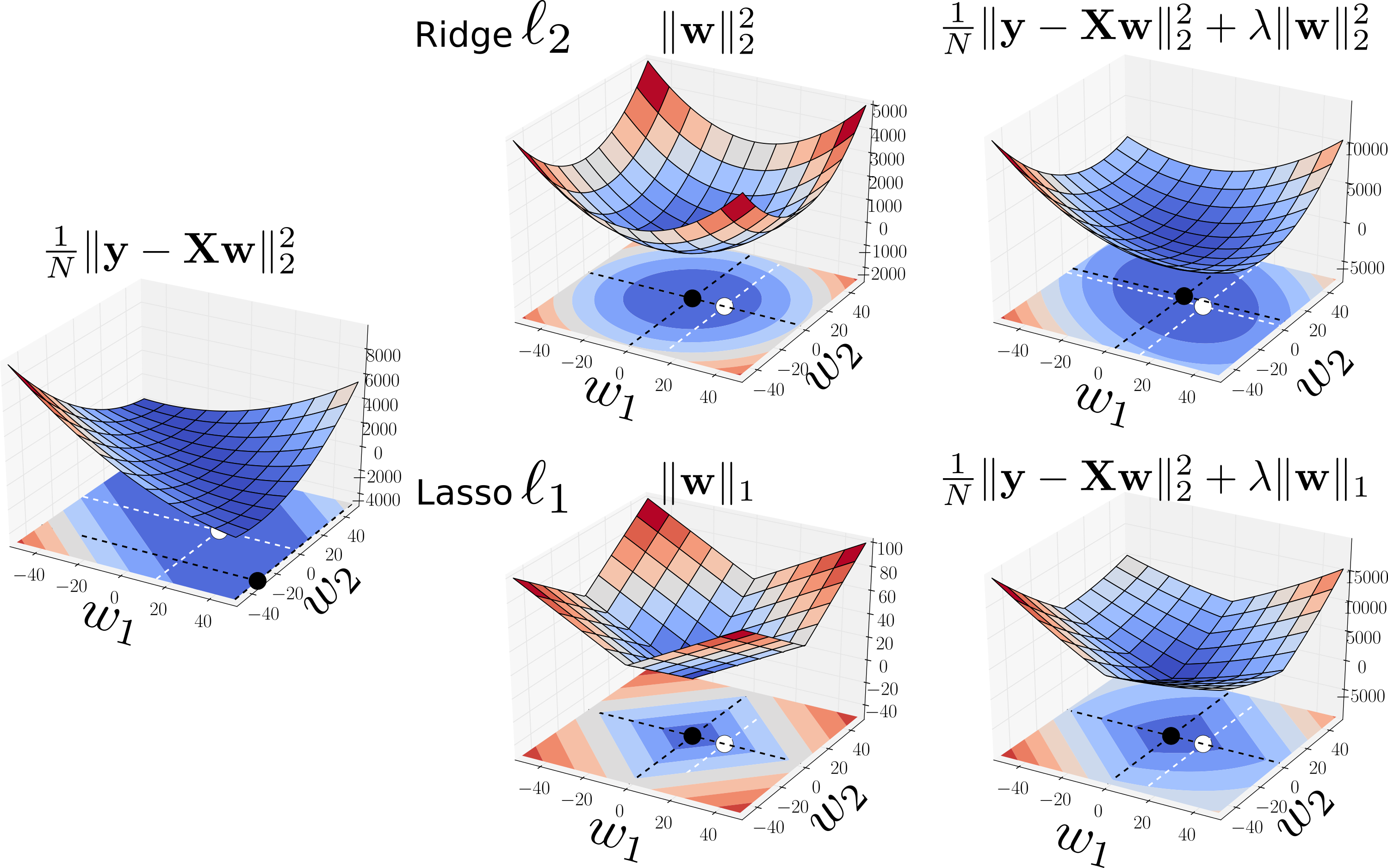
The ridge penalty shrinks the coefficients toward zero. The figure illustrates: the OLS solution on the left. The \(\ell_1\) and \(\ell_2\) penalties in the middle pane. The penalized OLS in the right pane. The right pane shows how the penalties shrink the coefficients toward zero. The black points are the minimum found in each case, and the white points represents the true solution used to generate the data.
\(\ell_1\) and \(\ell_2\) shrinkages
Elastic-net regression (\(\ell_1\)-\(\ell_2\)-regularization)
The Elastic-net estimator combines the \(\ell_1\) and \(\ell_2\) penalties, and results in the problem to
where \(\alpha\) acts as a global penalty and \(\rho\) as an \(\ell_1 / \ell_2\) ratio.
Rational
If there are groups of highly correlated variables, Lasso tends to arbitrarily select only one from each group. These models are difficult to interpret because covariates that are strongly associated with the outcome are not included in the predictive model. Conversely, the elastic net encourages a grouping effect, where strongly correlated predictors tend to be in or out of the model together.
Studies on real world data and simulation studies show that the elastic net often outperforms the lasso, while enjoying a similar sparsity of representation.
Regression performance evaluation metrics: R-squared, MSE and MAE
Common regression metrics are:
\(R^2\) : R-squared
MSE: Mean Squared Error
MAE: Mean Absolute Error
R-squared
The goodness of fit of a statistical model describes how well it fits a set of observations. Measures of goodness of fit typically summarize the discrepancy between observed values and the values expected under the model in question. We will consider the explained variance also known as the coefficient of determination, denoted \(R^2\) pronounced R-squared.
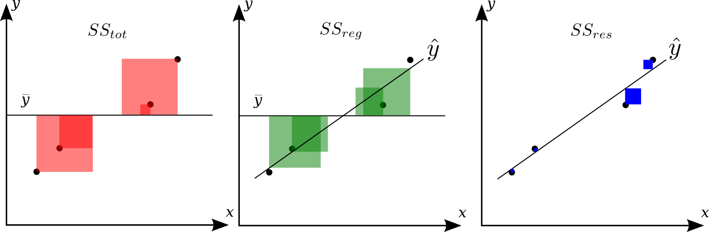
The total sum of squares, \(SS_\text{tot}\) is the sum of the sum of squares explained by the regression, \(SS_\text{reg}\), plus the sum of squares of residuals unexplained by the regression, \(SS_\text{res}\), also called the SSE, i.e. such that
title
The mean of \(y\) is
The total sum of squares is the total squared sum of deviations from the mean of \(y\), i.e.
The regression sum of squares, also called the explained sum of squares:
where \(\hat{y}_i = \beta x_i + \beta_0\) is the estimated value of salary \(\hat{y}_i\) given a value of experience \(x_i\).
The sum of squares of the residuals (SSE, Sum Squared Error), also called the residual sum of squares (RSS) is:
\(R^2\) is the explained sum of squares of errors. It is the variance explain by the regression divided by the total variance, i.e.
Test
Let \(\hat{\sigma}^2 = SS_\text{res} / (n-2)\) be an estimator of the variance of \(\epsilon\). The \(2\) in the denominator stems from the 2 estimated parameters: intercept and coefficient.
Unexplained variance: \(\frac{SS_\text{res}}{\hat{\sigma}^2} \sim \chi_{n-2}^2\)
Explained variance: \(\frac{SS_\text{reg}}{\hat{\sigma}^2} \sim \chi_{1}^2\). The single degree of freedom comes from the difference between \(\frac{SS_\text{tot}}{\hat{\sigma}^2} (\sim \chi^2_{n-1})\) and \(\frac{SS_\text{res}}{\hat{\sigma}^2} (\sim \chi_{n-2}^2)\), i.e. \((n-1) - (n-2)\) degree of freedom.
The Fisher statistics of the ratio of two variances:
Using the \(F\)-distribution, compute the probability of observing a value greater than \(F\) under \(H_0\), i.e.: \(P(x > F|H_0)\), i.e. the survival function \((1 - \text{Cumulative Distribution Function})\) at \(x\) of the given \(F\)-distribution.
import sklearn.metrics as metrics
from sklearn.model_selection import train_test_split

X, y = datasets.make_regression(random_state=0)
X_train, X_test, y_train, y_test = train_test_split(
    X, y, test_size=0.2, random_state=1)

lr = lm.LinearRegression()
lr.fit(X_train, y_train)
yhat = lr.predict(X_test)

r2 = metrics.r2_score(y_test, yhat)
mse = metrics.mean_squared_error(y_test, yhat)
mae = metrics.mean_absolute_error(y_test, yhat)

print("r2: %.3f, mae: %.3f, mse: %.3f" % (r2, mae, mse))
r2: 0.050, mae: 71.834, mse: 7891.217
In pure numpy:
res = y_test - lr.predict(X_test)

y_mu = np.mean(y_test)
ss_tot = np.sum((y_test - y_mu) ** 2)
ss_res = np.sum(res ** 2)

r2 = (1 - ss_res / ss_tot)
mse = np.mean(res ** 2)
mae = np.mean(np.abs(res))

print("r2: %.3f, mae: %.3f, mse: %.3f" % (r2, mae, mse))
r2: 0.050, mae: 71.834, mse: 7891.217