Linear dimension reduction and feature extraction

Introduction

In machine learning and statistics, dimensionality reduction or dimension reduction is the process of reducing the number of features under consideration, and can be divided into feature selection (not addressed here) and feature extraction.

Feature extraction starts from an initial set of measured data and builds derived values (features) intended to be informative and non-redundant, facilitating the subsequent learning and generalization steps, and in some cases leading to better human interpretations. Feature extraction is related to dimensionality reduction.

The input matrix \(\mathbf{X}\), of dimension \(N \times P\), is

\[\begin{split}\begin{bmatrix} x_{11} & \ldots & x_{1P}\\ & & \\ \vdots & \mathbf{X} & \vdots\\ & & \\ x_{N1} & \ldots & x_{NP} \end{bmatrix}\end{split}\]

where the rows represent the samples and columns represent the variables. The goal is to learn a transformation that extracts a few relevant features.

Models:

1. Linear matrix decomposition/factorisation SVD/PCA. Those models exploit the covariance \(\mathbf{\Sigma_{XX}}\) between the input features.

2. Non-linear models based on manifold learning: Isomap, t-SNE. Those models

Singular value decomposition and matrix factorization

Matrix factorization principles

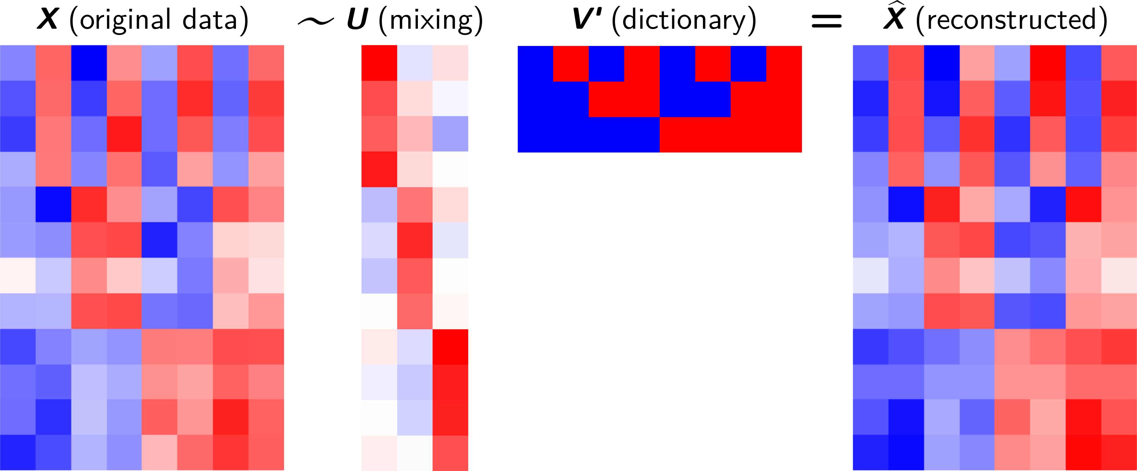
Decompose the data matrix \(\mathbf{X}_{N \times P}\) into a product of a mixing matrix \(\mathbf{U}_{N \times K}\) and a dictionary matrix \(\mathbf{V}_{P \times K}\).

\[\mathbf{X} = \mathbf{U} \mathbf{V}^{T},\]

If we consider only a subset of components \(K<rank(\mathbf{X}) < \min(P, N-1)\) , \(\mathbf{X}\) is approximated by a matrix \(\hat{\mathbf{X}}\):

\[\mathbf{X} \approx \hat{\mathbf{X}} = \mathbf{U} \mathbf{V}^{T},\]

Each line of \(\mathbf{x_i}\) is a linear combination (mixing \(\mathbf{u_i}\)) of dictionary items \(\mathbf{V}\).

\(N\) \(P\)-dimensional data points lie in a space whose dimension is less than \(N-1\) (2 dots lie on a line, 3 on a plane, etc.).

Matrix factorization

Singular value decomposition (SVD) principles

Singular-value decomposition (SVD) factorises the data matrix \(\mathbf{X}_{N \times P}\) into a product:

\[\mathbf{X} = \mathbf{U}\mathbf{D}\mathbf{V}^{T},\]

where

\[\begin{split}\begin{bmatrix} x_{11} & & x_{1P}\\ & & \\ & \mathbf{X} & \\ & & \\ x_{N1} & & x_{NP} \end{bmatrix} = \begin{bmatrix} u_{11} & & u_{1K}\\ & & \\ & \mathbf{U} & \\ & & \\ u_{N1} & & u_{NK} \end{bmatrix} \begin{bmatrix} d_{1}& & 0\\ & \mathbf{D} &\\ 0 & & d_{K} \end{bmatrix} \begin{bmatrix} v_{11}& & v_{1P}\\ & \mathbf{V}^T & \\ v_{K1}& & v_{KP} \end{bmatrix}.\end{split}\]

\(\mathbf{U}\): right-singular

• \(\mathbf{V} = [\mathbf{v}_1,\cdots , \mathbf{v}_K]\) is a \(P \times K\) orthogonal matrix.

• It is a dictionary of patterns to be combined (according to the mixing coefficients) to reconstruct the original samples.

• \(\mathbf{V}\) perfoms the initial rotations (projection) along the \(K=\min(N, P)\) principal component directions, also called loadings.

• Each \(\mathbf{v}_j\) performs the linear combination of the variables that has maximum sample variance, subject to being uncorrelated with the previous \(\mathbf{v}_{j-1}\).

\(\mathbf{D}\): singular values

• \(\mathbf{D}\) is a \(K \times K\) diagonal matrix made of the singular values of \(\mathbf{X}\) with \(d_1 \geq d_2 \geq \cdots \geq d_K \geq 0\).

• \(\mathbf{D}\) scale the projection along the coordinate axes by \(d_1, d_2, \cdots, d_K\).

• Singular values are the square roots of the eigenvalues of \(\mathbf{X}^{T}\mathbf{X}\).

\(\mathbf{V}\): left-singular vectors

• \(\mathbf{U} = [\mathbf{u}_1, \cdots , \mathbf{u}_K]\) is an \(N \times K\) orthogonal matrix.

• Each row \(\mathbf{v_i}\) provides the mixing coefficients of dictionary items to reconstruct the sample \(\mathbf{x_i}\)

• It may be understood as the coordinates on the new orthogonal basis (obtained after the initial rotation) called principal components in the PCA.

SVD for variables transformation

\(\mathbf{V}\) transforms correlated variables (\(\mathbf{X}\)) into a set of uncorrelated ones (\(\mathbf{U}\mathbf{D}\)) that better expose the various relationships among the original data items.

At the same time, SVD is a method for identifying and ordering the dimensions along which data points exhibit the most variation.

import numpy as np
import scipy
from sklearn.decomposition import PCA
import matplotlib.pyplot as plt
import seaborn as sns
%matplotlib inline

np.random.seed(42)

# dataset
n_samples = 100
experience = np.random.normal(size=n_samples)
salary = 1500 + experience + np.random.normal(size=n_samples, scale=.5)
X = np.column_stack([experience, salary])
print(X.shape)

# PCA using SVD
X -= X.mean(axis=0)  # Centering is required
U, s, Vh = scipy.linalg.svd(X, full_matrices=False)
# U : Unitary matrix having left singular vectors as columns.
#     Of shape (n_samples,n_samples) or (n_samples,n_comps), depending on
#     full_matrices.
#
# s : The singular values, sorted in non-increasing order. Of shape (n_comps,),
#     with n_comps = min(n_samples, n_features).
#
# Vh: Unitary matrix having right singular vectors as rows.
#     Of shape (n_features, n_features) or (n_comps, n_features) depending
# on full_matrices.

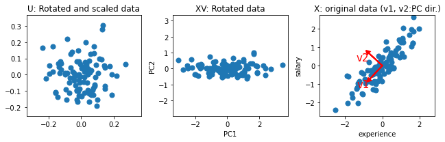
plt.figure(figsize=(9, 3))

plt.subplot(131)
plt.scatter(U[:, 0], U[:, 1], s=50)
plt.axis('equal')
plt.title("U: Rotated and scaled data")

plt.subplot(132)

# Project data
PC = np.dot(X, Vh.T)
plt.scatter(PC[:, 0], PC[:, 1], s=50)
plt.axis('equal')
plt.title("XV: Rotated data")
plt.xlabel("PC1")
plt.ylabel("PC2")

plt.subplot(133)
plt.scatter(X[:, 0], X[:, 1], s=50)
for i in range(Vh.shape[0]):
    plt.arrow(x=0, y=0, dx=Vh[i, 0], dy=Vh[i, 1], head_width=0.2,
              head_length=0.2, linewidth=2, fc='r', ec='r')
    plt.text(Vh[i, 0], Vh[i, 1],'v%i' % (i+1), color="r", fontsize=15,
             horizontalalignment='right', verticalalignment='top')
plt.axis('equal')
plt.ylim(-4, 4)

plt.title("X: original data (v1, v2:PC dir.)")
plt.xlabel("experience")
plt.ylabel("salary")

plt.tight_layout()

(100, 2)

Principal components analysis (PCA)

Sources:

• C. M. Bishop Pattern Recognition and Machine Learning, Springer, 2006

• Everything you did and didn’t know about PCA

• Principal Component Analysis in 3 Simple Steps

Principles

• Principal components analysis is the main method used for linear dimension reduction.

• The idea of principal component analysis is to find the \(K\) principal components directions (called the loadings) \(\mathbf{V}_{K\times P}\) that capture the variation in the data as much as possible.

• It converts a set of \(N\) \(P\)-dimensional observations \(\mathbf{N}_{N\times P}\) of possibly correlated variables into a set of \(N\) \(K\)-dimensional samples \(\mathbf{C}_{N\times K}\), where the \(K < P\). The new variables are linearly uncorrelated. The columns of \(\mathbf{C}_{N\times K}\) are called the principal components.

• The dimension reduction is obtained by using only \(K < P\) components that exploit correlation (covariance) among the original variables.

• PCA is mathematically defined as an orthogonal linear transformation \(\mathbf{V}_{K\times P}\) that transforms the data to a new coordinate system such that the greatest variance by some projection of the data comes to lie on the first coordinate (called the first principal component), the second greatest variance on the second coordinate, and so on.

  \[\mathbf{C}_{N\times K} = \mathbf{X}_{N \times P} \mathbf{V}_{P \times K}\]

• PCA can be thought of as fitting a \(P\)-dimensional ellipsoid to the data, where each axis of the ellipsoid represents a principal component. If some axis of the ellipse is small, then the variance along that axis is also small, and by omitting that axis and its corresponding principal component from our representation of the dataset, we lose only a commensurately small amount of information.

• Finding the \(K\) largest axes of the ellipse will permit to project the data onto a space having dimensionality \(K < P\) while maximizing the variance of the projected data.

Dataset preprocessing

Centering

Consider a data matrix, \(\mathbf{X}\) , with column-wise zero empirical mean (the sample mean of each column has been shifted to zero), ie. \(\mathbf{X}\) is replaced by \(\mathbf{X} - \mathbf{1}\bar{\mathbf{x}}^T\).

Standardizing

Optionally, standardize the columns, i.e., scale them by their standard-deviation. Without standardization, a variable with a high variance will capture most of the effect of the PCA. The principal direction will be aligned with this variable. Standardization will, however, raise noise variables to the save level as informative variables.

The covariance matrix of centered standardized data is the correlation matrix.

Eigendecomposition of the data covariance matrix

To begin with, consider the projection onto a one-dimensional space (\(K = 1\)). We can define the direction of this space using a \(P\)-dimensional vector \(\mathbf{v}\), which for convenience (and without loss of generality) we shall choose to be a unit vector so that \(\|\mathbf{v}\|_2 = 1\) (note that we are only interested in the direction defined by \(\mathbf{v}\), not in the magnitude of \(\mathbf{v}\) itself). PCA consists of two mains steps:

Projection in the directions that capture the greatest variance

Each \(P\)-dimensional data point \(\mathbf{x}_i\) is then projected onto \(\mathbf{v}\), where the coordinate (in the coordinate system of \(\mathbf{v}\)) is a scalar value, namely \(\mathbf{x}_i^T \mathbf{v}\). I.e., we want to find the vector \(\mathbf{v}\) that maximizes these coordinates along \(\mathbf{v}\), which we will see corresponds to maximizing the variance of the projected data. This is equivalently expressed as

\[\mathbf{v} = \arg \max_{\|\mathbf{v}\|=1}\frac{1}{N}\sum_i \left(\mathbf{x}_i^T \mathbf{v}\right)^2.\]

We can write this in matrix form as

\[\mathbf{v} = \arg \max_{\|\mathbf{v}\|=1} \frac{1}{N} \|\mathbf{X} \mathbf{v}\|^2 = \frac{1}{N} \mathbf{v}^T \mathbf{X}^T \mathbf{X} \mathbf{v} = \mathbf{v}^T\mathbf{S_{XX}}\mathbf{v},\]

where \(\mathbf{S_{XX}}\) is a biased estiamte of the covariance matrix of the data, i.e.

\[\mathbf{S_{XX}} = \frac{1}{N} \mathbf{X}^T\mathbf{X}.\]

We now maximize the projected variance \(\mathbf{v}^T \mathbf{S_{XX}} \mathbf{v}\) with respect to \(\mathbf{v}\). Clearly, this has to be a constrained maximization to prevent \(\|\mathbf{v}_2\| \rightarrow \infty\). The appropriate constraint comes from the normalization condition \(\|\mathbf{v}\|_2 \equiv \|\mathbf{v}\|_2^2 = \mathbf{v}^T \mathbf{v} = 1\). To enforce this constraint, we introduce a Lagrange multiplier that we shall denote by \(\lambda\), and then make an unconstrained maximization of

\[\mathbf{v}^T\mathbf{S_{XX}} \mathbf{v} - \lambda (\mathbf{v}^T \mathbf{v} - 1).\]

By setting the gradient with respect to \(\mathbf{v}\) equal to zero, we see that this quantity has a stationary point when

\[\mathbf{S_{XX}} \mathbf{v} = \lambda \mathbf{v}.\]

We note that \(\mathbf{v}\) is an eigenvector of \(\mathbf{S_{XX}}\).

If we left-multiply the above equation by \(\mathbf{v}^T\) and make use of \(\mathbf{v}^T \mathbf{v} = 1\), we see that the variance is given by

\[\mathbf{v}^T \mathbf{S_{XX}} \mathbf{v} = \lambda,\]

and so the variance will be at a maximum when \(\mathbf{v}\) is equal to the eigenvector corresponding to the largest eigenvalue, \(\lambda\). This eigenvector is known as the first principal component.

We can define additional principal components in an incremental fashion by choosing each new direction to be that which maximizes the projected variance amongst all possible directions that are orthogonal to those already considered. If we consider the general case of a \(K\)-dimensional projection space, the optimal linear projection for which the variance of the projected data is maximized is now defined by the \(K\) eigenvectors, \(\mathbf{v_1}, \ldots , \mathbf{v_K}\), of the data covariance matrix \(\mathbf{S_{XX}}\) that corresponds to the \(K\) largest eigenvalues, \(\lambda_1 \geq \lambda_2 \geq \cdots \geq \lambda_K\).

Back to SVD

The sample covariance matrix of centered data \(\mathbf{X}\) is given by

\[\mathbf{S_{XX}} = \frac{1}{N-1}\mathbf{X}^T\mathbf{X}.\]

We rewrite \(\mathbf{X}^T\mathbf{X}\) using the SVD decomposition of \(\mathbf{X}\) as

Considering only the \(k^{th}\) right-singular vectors \(\mathbf{v}_k\) associated to the singular value \(d_k\)

\[\mathbf{v_k}^T\mathbf{S_{XX}}\mathbf{v_k} = \frac{1}{N-1}d_k^2,\]

It turns out that if you have done the singular value decomposition then you already have the Eigenvalue decomposition for \(\mathbf{X}^T\mathbf{X}\). Where - The eigenvectors of \(\mathbf{S_{XX}}\) are equivalent to the right singular vectors, \(\mathbf{V}\), of \(\mathbf{X}\). - The eigenvalues, \(\lambda_k\), of \(\mathbf{S_{XX}}\), i.e. the variances of the components, are equal to \(\frac{1}{N-1}\) times the squared singular values, \(d_k\).

Moreover computing PCA with SVD do not require to form the matrix \(\mathbf{X}^T\mathbf{X}\), so computing the SVD is now the standard way to calculate a principal components analysis from a data matrix, unless only a handful of components are required.

PCA outputs

The SVD or the eigendecomposition of the data covariance matrix provides three main quantities:

1. Principal component directions or loadings are the eigenvectors of \(\mathbf{X}^T\mathbf{X}\). The \(\mathbf{V}_{K \times P}\) or the right-singular vectors of an SVD of \(\mathbf{X}\) are called principal component directions of \(\mathbf{X}\). They are generally computed using the SVD of \(\mathbf{X}\).

2. Principal components is the \({N\times K}\) matrix \(\mathbf{C}\) which is obtained by projecting \(\mathbf{X}\) onto the principal components directions, i.e.

\[\mathbf{C}_{N\times K} = \mathbf{X}_{N \times P} \mathbf{V}_{P \times K}.\]

Since \(\mathbf{X} = \mathbf{UDV}^T\) and \(\mathbf{V}\) is orthogonal (\(\mathbf{V}^T \mathbf{V} = \mathbf{I}\)):

Thus \(\mathbf{c}_j = \mathbf{X}\mathbf{v}_j = \mathbf{u}_j d_j\), for \(j=1, \ldots K\). Hence \(\mathbf{u}_j\) is simply the projection of the row vectors of \(\mathbf{X}\), i.e., the input predictor vectors, on the direction \(\mathbf{v}_j\), scaled by \(d_j\).

\[\begin{split}\mathbf{c}_1= \begin{bmatrix} x_{1,1}v_{1,1}+ \ldots +x_{1,P}v_{1,P}\\ x_{2,1}v_{1,1}+ \ldots +x_{2,P}v_{1,P}\\ \vdots\\ x_{N,1}v_{1,1}+ \ldots +x_{N,P}v_{1,P} \end{bmatrix}\end{split}\]

3. The variance of each component is given by the eigen values \(\lambda_k, k=1, \dots K\). It can be obtained from the singular values:

Determining the number of PCs

We must choose \(K^* \in [1, \ldots, K]\), the number of required components. This can be done by calculating the explained variance ratio of the \(K^*\) first components and by choosing \(K^*\) such that the cumulative explained variance ratio is greater than some given threshold (e.g., \(\approx 90\%\)). This is expressed as

\[\mathrm{cumulative~explained~variance}(\mathbf{c}_k) = \frac{\sum_j^{K^*} var(\mathbf{c}_k)}{\sum_j^K var(\mathbf{c}_k)}.\]

Interpretation and visualization

PCs

Plot the samples projeted on first the principal components as e.g. PC1 against PC2.

PC directions

Exploring the loadings associated with a component provides the contribution of each original variable in the component.

Remark: The loadings (PC directions) are the coefficients of multiple regression of PC on original variables:

Another way to evaluate the contribution of the original variables in each PC can be obtained by computing the correlation between the PCs and the original variables, i.e. columns of \(\mathbf{X}\), denoted \(\mathbf{x}_j\), for \(j=1, \ldots, P\). For the \(k^{th}\) PC, compute and plot the correlations with all original variables

\[cor(\mathbf{c}_k, \mathbf{x}_j), j=1 \ldots K, j=1 \ldots K.\]

These quantities are sometimes called the correlation loadings.

import numpy as np
from sklearn.decomposition import PCA
import matplotlib.pyplot as plt

np.random.seed(42)

# dataset
n_samples = 100
experience = np.random.normal(size=n_samples)
salary = 1500 + experience + np.random.normal(size=n_samples, scale=.5)
X = np.column_stack([experience, salary])

# PCA with scikit-learn
pca = PCA(n_components=2)
pca.fit(X)
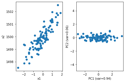
print(pca.explained_variance_ratio_)

PC = pca.transform(X)

plt.subplot(121)
plt.scatter(X[:, 0], X[:, 1])
plt.xlabel("x1"); plt.ylabel("x2")

plt.subplot(122)
plt.scatter(PC[:, 0], PC[:, 1])
plt.xlabel("PC1 (var=%.2f)" % pca.explained_variance_ratio_[0])
plt.ylabel("PC2 (var=%.2f)" % pca.explained_variance_ratio_[1])
plt.axis('equal')
plt.tight_layout()

[0.93646607 0.06353393]

from time import time
import numpy as np
import matplotlib.pyplot as plt
from matplotlib import offsetbox
from sklearn import (manifold, datasets, decomposition, ensemble,
                     discriminant_analysis, random_projection, neighbors)
print(__doc__)

digits = datasets.load_digits(n_class=6)
X = digits.data
y = digits.target
n_samples, n_features = X.shape
n_neighbors = 30

Automatically created module for IPython interactive environment

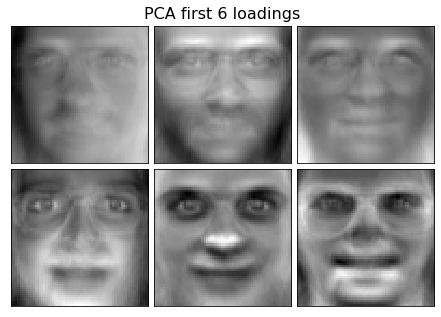
Eigen faces

Sources: Scikit learn Faces decompositions

Load data

import matplotlib.pyplot as plt
from sklearn.datasets import fetch_olivetti_faces
from sklearn import decomposition

n_row, n_col = 2, 3
n_components = n_row * n_col
image_shape = (64, 64)

faces, _ = fetch_olivetti_faces(return_X_y=True, shuffle=True,
                                random_state=1)
n_samples, n_features = faces.shape


# Utils function
def plot_gallery(title, images, n_col=n_col, n_row=n_row, cmap=plt.cm.gray):
    plt.figure(figsize=(2. * n_col, 2.26 * n_row))
    plt.suptitle(title, size=16)
    for i, comp in enumerate(images):
        plt.subplot(n_row, n_col, i + 1)
        vmax = max(comp.max(), -comp.min())
        plt.imshow(comp.reshape(image_shape), cmap=cmap,
                   interpolation='nearest',
                   vmin=-vmax, vmax=vmax)
        plt.xticks(())
        plt.yticks(())
    plt.subplots_adjust(0.01, 0.05, 0.99, 0.93, 0.04, 0.)

Preprocessing

# global centering
faces_centered = faces - faces.mean(axis=0)

# local centering
faces_centered -= faces_centered.mean(axis=1).reshape(n_samples, -1)

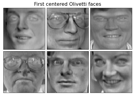
First centered Olivetti faces

plot_gallery("First centered Olivetti faces", faces_centered[:n_components])

pca = decomposition.PCA(n_components=n_components)
pca.fit(faces_centered)
plot_gallery("PCA first %i loadings" % n_components, pca.components_[:n_components])

Exercises

Write a basic PCA class

Write a class BasicPCA with two methods:

• fit(X) that estimates the data mean, principal components directions \(\textbf{V}\) and the explained variance of each component.

• transform(X) that projects the data onto the principal components.

Check that your BasicPCA gave similar results, compared to the results from sklearn.

Apply your Basic PCA on the iris dataset

The data set is available at: https://github.com/duchesnay/pystatsml/raw/master/datasets/iris.csv

• Describe the data set. Should the dataset been standardized?

• Describe the structure of correlations among variables.

• Compute a PCA with the maximum number of components.

• Compute the cumulative explained variance ratio. Determine the number of components \(K\) by your computed values.

• Print the \(K\) principal components directions and correlations of the \(K\) principal components with the original variables. Interpret the contribution of the original variables into the PC.

• Plot the samples projected into the \(K\) first PCs.

• Color samples by their species.

Run scikit-learn examples

Load the notebook or python file at the end of each examples

• Faces dataset decompositions

• Faces recognition example using eigenfaces and SVMs