Multilayer Perceptron (MLP)
Course outline:
Recall of linear classifier
MLP with scikit-learn
MLP with pytorch
Test several MLP architectures
Limits of MLP
Sources:
Deep learning
Pytorch
MNIST and pytorch:
%matplotlib inline

import os
import numpy as np
import torch
import torch.nn as nn
import torch.nn.functional as F
import torch.optim as optim
from torch.optim import lr_scheduler
import torchvision
from torchvision import transforms
from torchvision import datasets
from torchvision import models
#
from pathlib import Path
import matplotlib.pyplot as plt

# Device configuration
device = torch.device('cuda:0' if torch.cuda.is_available() else 'cpu')
device = 'cpu' # Force CPU
print(device)
cpu
Hyperparameters
Dataset: MNIST Handwritten Digit Recognition
from pathlib import Path
WD = os.path.join(Path.home(), "data", "pystatml", "dl_mnist_pytorch")
os.makedirs(WD, exist_ok=True)
os.chdir(WD)
print("Working dir is:", os.getcwd())
os.makedirs("data", exist_ok=True)
os.makedirs("models", exist_ok=True)

def load_mnist(batch_size_train, batch_size_test):

    train_loader = torch.utils.data.DataLoader(
        datasets.MNIST('data', train=True, download=True,
                       transform=transforms.Compose([
                           transforms.ToTensor(),
                           transforms.Normalize((0.1307,), (0.3081,)) # Mean and Std of the MNIST dataset
                       ])),
        batch_size=batch_size_train, shuffle=True)

    val_loader = torch.utils.data.DataLoader(
        datasets.MNIST('data', train=False, transform=transforms.Compose([
            transforms.ToTensor(),
            transforms.Normalize((0.1307,), (0.3081,)) # Mean and Std of the MNIST dataset
        ])),
        batch_size=batch_size_test, shuffle=True)
    return train_loader, val_loader


train_loader, val_loader = load_mnist(64, 10000)

dataloaders = dict(train=train_loader, val=val_loader)

# Info about the dataset
D_in = np.prod(dataloaders["train"].dataset.data.shape[1:])
D_out = len(dataloaders["train"].dataset.targets.unique())
print("Datasets shapes:", {x: dataloaders[x].dataset.data.shape for x in ['train', 'val']})
print("N input features:", D_in, "Output classes:", D_out)
Working dir is: /home/ed203246/data/pystatml/dl_mnist_pytorch
Datasets shapes: {'train': torch.Size([60000, 28, 28]), 'val': torch.Size([10000, 28, 28])}
N input features: 784 Output classes: 10
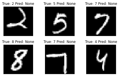
Now let’s take a look at some mini-batches examples.
batch_idx, (example_data, example_targets) = next(enumerate(train_loader))
print("Train batch:", example_data.shape, example_targets.shape)
batch_idx, (example_data, example_targets) = next(enumerate(val_loader))
print("Val batch:", example_data.shape, example_targets.shape)
Train batch: torch.Size([64, 1, 28, 28]) torch.Size([64])
Val batch: torch.Size([10000, 1, 28, 28]) torch.Size([10000])
So one test data batch is a tensor of shape: . This means we have 1000 examples of 28x28 pixels in grayscale (i.e. no rgb channels, hence the one). We can plot some of them using matplotlib.
def show_data_label_prediction(data, y_true, y_pred=None, shape=(2, 3)):
    y_pred = [None] * len(y_true) if y_pred is None else y_pred
    fig = plt.figure()
    for i in range(np.prod(shape)):
        plt.subplot(*shape, i+1)
        plt.tight_layout()
        plt.imshow(data[i][0], cmap='gray', interpolation='none')
        plt.title("True: {} Pred: {}".format(y_true[i], y_pred[i]))
        plt.xticks([])
        plt.yticks([])

show_data_label_prediction(data=example_data, y_true=example_targets, y_pred=None, shape=(2, 3))
Recall of linear classifier
Binary logistic regression
1 neuron as output layer
Softmax Classifier (Multinomial Logistic Regression)
Input \(x\): a vector of dimension \((0)\) (layer 0).
Ouput \(f(x)\) a vector of \((1)\) (layer 1) possible labels
The model as \((1)\) neurons as output layer
Where \(W\) is a \((0) \times (1)\) of coefficients and \(b\) is a \((1)\)-dimentional vector of bias.
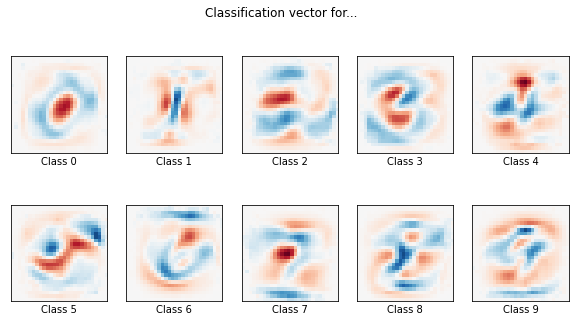
MNIST classfification using multinomial logistic
source: Logistic regression MNIST
Here we fit a multinomial logistic regression with L2 penalty on a subset of the MNIST digits classification task.
X_train = train_loader.dataset.data.numpy()
#print(X_train.shape)
X_train = X_train.reshape((X_train.shape[0], -1))
y_train = train_loader.dataset.targets.numpy()

X_test = val_loader.dataset.data.numpy()
X_test = X_test.reshape((X_test.shape[0], -1))
y_test = val_loader.dataset.targets.numpy()

print(X_train.shape, y_train.shape)
(60000, 784) (60000,)
import matplotlib.pyplot as plt
import numpy as np

#from sklearn.datasets import fetch_openml
from sklearn.linear_model import LogisticRegression
#from sklearn.model_selection import train_test_split
from sklearn.preprocessing import StandardScaler
from sklearn.utils import check_random_state

scaler = StandardScaler()
X_train = scaler.fit_transform(X_train)
X_test = scaler.transform(X_test)

# Turn up tolerance for faster convergence
clf = LogisticRegression(C=50., multi_class='multinomial', solver='sag', tol=0.1)
clf.fit(X_train, y_train)
#sparsity = np.mean(clf.coef_ == 0) * 100
score = clf.score(X_test, y_test)

print("Test score with penalty: %.4f" % score)
Test score with penalty: 0.8997
coef = clf.coef_.copy()
plt.figure(figsize=(10, 5))
scale = np.abs(coef).max()
for i in range(10):
    l1_plot = plt.subplot(2, 5, i + 1)
    l1_plot.imshow(coef[i].reshape(28, 28), interpolation='nearest',
                   cmap=plt.cm.RdBu, vmin=-scale, vmax=scale)
    l1_plot.set_xticks(())
    l1_plot.set_yticks(())
    l1_plot.set_xlabel('Class %i' % i)
plt.suptitle('Classification vector for...')

plt.show()
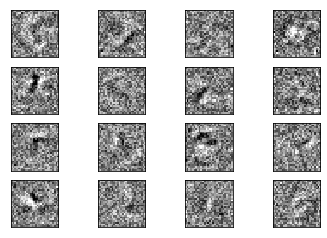
Model: Two Layer MLP
MLP with Scikit-learn
from sklearn.neural_network import MLPClassifier

mlp = MLPClassifier(hidden_layer_sizes=(100, ), max_iter=5, alpha=1e-4,
                    solver='sgd', verbose=10, tol=1e-4, random_state=1,
                    learning_rate_init=0.01, batch_size=64)

mlp.fit(X_train, y_train)
print("Training set score: %f" % mlp.score(X_train, y_train))
print("Test set score: %f" % mlp.score(X_test, y_test))

print("Coef shape=", len(mlp.coefs_))

fig, axes = plt.subplots(4, 4)
# use global min / max to ensure all weights are shown on the same scale
vmin, vmax = mlp.coefs_[0].min(), mlp.coefs_[0].max()
for coef, ax in zip(mlp.coefs_[0].T, axes.ravel()):
    ax.matshow(coef.reshape(28, 28), cmap=plt.cm.gray, vmin=.5 * vmin,
               vmax=.5 * vmax)
    ax.set_xticks(())
    ax.set_yticks(())

plt.show()
Iteration 1, loss = 0.28828673
Iteration 2, loss = 0.13388073
Iteration 3, loss = 0.09366379
Iteration 4, loss = 0.07317648
Iteration 5, loss = 0.05340251
/home/ed203246/anaconda3/lib/python3.7/site-packages/sklearn/neural_network/_multilayer_perceptron.py:585: ConvergenceWarning: Stochastic Optimizer: Maximum iterations (5) reached and the optimization hasn't converged yet.
  % self.max_iter, ConvergenceWarning)
Training set score: 0.989067
Test set score: 0.971900
Coef shape= 2
MLP with pytorch
class TwoLayerMLP(nn.Module):

    def __init__(self, d_in, d_hidden, d_out):
        super(TwoLayerMLP, self).__init__()
        self.d_in = d_in

        self.linear1 = nn.Linear(d_in, d_hidden)
        self.linear2 = nn.Linear(d_hidden, d_out)

    def forward(self, X):
        X = X.view(-1, self.d_in)
        X = self.linear1(X)
        return F.log_softmax(self.linear2(X), dim=1)
Train the Model
First we want to make sure our network is in training mode.
Iterate over epochs
Alternate train and validation dataset
Iterate over all training/val data once per epoch. Loading the individual batches is handled by the DataLoader.
Set the gradients to zero using
optimizer.zero_grad()since PyTorch by default accumulates gradients.Forward pass:
model(inputs): Produce the output of our network.torch.max(outputs, 1): softmax predictions.criterion(outputs, labels): loss between the output and the ground truth label.
In training mode, backward pass
backward(): collect a new set of gradients which we propagate back into each of the network’s parameters usingoptimizer.step().We’ll also keep track of the progress with some printouts. In order to create a nice training curve later on we also create two lists for saving training and testing losses. On the x-axis we want to display the number of training examples the network has seen during training.
Save model state: Neural network modules as well as optimizers have the ability to save and load their internal state using
.state_dict(). With this we can continue training from previously saved state dicts if needed - we’d just need to call.load_state_dict(state_dict).
# %load train_val_model.py
# %load train_val_model.py
import numpy as np
import torch
import time
import copy


def train_val_model(model, criterion, optimizer, dataloaders, num_epochs=25,
        scheduler=None, log_interval=None):
    since = time.time()

    best_model_wts = copy.deepcopy(model.state_dict())
    best_acc = 0.0

    # Store losses and accuracies accross epochs
    losses, accuracies = dict(train=[], val=[]), dict(train=[], val=[])

    for epoch in range(num_epochs):
        if log_interval is not None and epoch % log_interval == 0:
            print('Epoch {}/{}'.format(epoch, num_epochs - 1))
            print('-' * 10)

        # Each epoch has a training and validation phase
        for phase in ['train', 'val']:
            if phase == 'train':
                model.train()  # Set model to training mode
            else:
                model.eval()   # Set model to evaluate mode

            running_loss = 0.0
            running_corrects = 0

            # Iterate over data.
            nsamples = 0
            for inputs, labels in dataloaders[phase]:
                inputs = inputs.to(device)
                labels = labels.to(device)
                nsamples += inputs.shape[0]

                # zero the parameter gradients
                optimizer.zero_grad()

                # forward
                # track history if only in train
                with torch.set_grad_enabled(phase == 'train'):
                    outputs = model(inputs)
                    _, preds = torch.max(outputs, 1)
                    loss = criterion(outputs, labels)

                    # backward + optimize only if in training phase
                    if phase == 'train':
                        loss.backward()
                        optimizer.step()

                # statistics
                running_loss += loss.item() * inputs.size(0)
                running_corrects += torch.sum(preds == labels.data)

            if scheduler is not None and phase == 'train':
                scheduler.step()

            #nsamples = dataloaders[phase].dataset.data.shape[0]
            epoch_loss = running_loss / nsamples
            epoch_acc = running_corrects.double() / nsamples

            losses[phase].append(epoch_loss)
            accuracies[phase].append(epoch_acc)
            if log_interval is not None and epoch % log_interval == 0:
                print('{} Loss: {:.4f} Acc: {:.2f}%'.format(
                    phase, epoch_loss, 100 * epoch_acc))

            # deep copy the model
            if phase == 'val' and epoch_acc > best_acc:
                best_acc = epoch_acc
                best_model_wts = copy.deepcopy(model.state_dict())
        if log_interval is not None and epoch % log_interval == 0:
            print()

    time_elapsed = time.time() - since
    print('Training complete in {:.0f}m {:.0f}s'.format(
        time_elapsed // 60, time_elapsed % 60))
    print('Best val Acc: {:.2f}%'.format(100 * best_acc))

    # load best model weights
    model.load_state_dict(best_model_wts)

    return model, losses, accuracies
Run one epoch and save the model
model = TwoLayerMLP(D_in, 50, D_out).to(device)
print(next(model.parameters()).is_cuda)
optimizer = optim.SGD(model.parameters(), lr=0.01, momentum=0.5)
criterion = nn.NLLLoss()

# Explore the model
for parameter in model.parameters():
    print(parameter.shape)

print("Total number of parameters =", np.sum([np.prod(parameter.shape) for parameter in model.parameters()]))

model, losses, accuracies = train_val_model(model, criterion, optimizer, dataloaders,
                       num_epochs=1, log_interval=1)

print(next(model.parameters()).is_cuda)
torch.save(model.state_dict(), 'models/mod-%s.pth' % model.__class__.__name__)
False
torch.Size([50, 784])
torch.Size([50])
torch.Size([10, 50])
torch.Size([10])
Total number of parameters = 39760
Epoch 0/0
----------
train Loss: 0.4431 Acc: 87.93%
val Loss: 0.3062 Acc: 91.21%

Training complete in 0m 7s
Best val Acc: 91.21%
False
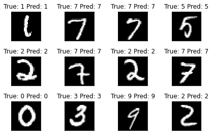
Use the model to make new predictions. Consider the device, ie, load
data on device example_data.to(device) from prediction, then move
back to cpu example_data.cpu().
batch_idx, (example_data, example_targets) = next(enumerate(val_loader))
example_data = example_data.to(device)

with torch.no_grad():
  output = model(example_data).cpu()

example_data = example_data.cpu()

# print(output.is_cuda)

# Softmax predictions
preds = output.argmax(dim=1)

print("Output shape=", output.shape, "label shape=", preds.shape)
print("Accuracy = {:.2f}%".format((example_targets == preds).sum().item() * 100. / len(example_targets)))

show_data_label_prediction(data=example_data, y_true=example_targets, y_pred=preds, shape=(3, 4))
Output shape= torch.Size([10000, 10]) label shape= torch.Size([10000])
Accuracy = 91.21%
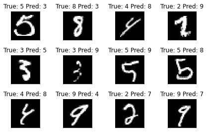
Plot missclassified samples
errors = example_targets != preds
#print(errors, np.where(errors))
print("Nb errors = {}, (Error rate = {:.2f}%)".format(errors.sum(), 100 * errors.sum().item() / len(errors)))
err_idx = np.where(errors)[0]
show_data_label_prediction(data=example_data[err_idx], y_true=example_targets[err_idx],
                           y_pred=preds[err_idx], shape=(3, 4))
Nb errors = 879, (Error rate = 8.79%)
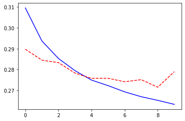
Continue training from checkpoints: reload the model and run 10 more epochs
model = TwoLayerMLP(D_in, 50, D_out)
model.load_state_dict(torch.load('models/mod-%s.pth' % model.__class__.__name__))
model.to(device)

optimizer = optim.SGD(model.parameters(), lr=0.01, momentum=0.5)
criterion = nn.NLLLoss()

model, losses, accuracies = train_val_model(model, criterion, optimizer, dataloaders,
                       num_epochs=10, log_interval=2)

_ = plt.plot(losses['train'], '-b', losses['val'], '--r')
Epoch 0/9
----------
train Loss: 0.3096 Acc: 91.11%
val Loss: 0.2897 Acc: 91.65%

Epoch 2/9
----------
train Loss: 0.2853 Acc: 92.03%
val Loss: 0.2833 Acc: 92.04%

Epoch 4/9
----------
train Loss: 0.2749 Acc: 92.36%
val Loss: 0.2757 Acc: 92.01%

Epoch 6/9
----------
train Loss: 0.2692 Acc: 92.51%
val Loss: 0.2741 Acc: 92.29%

Epoch 8/9
----------
train Loss: 0.2651 Acc: 92.61%
val Loss: 0.2715 Acc: 92.32%

Training complete in 1m 14s
Best val Acc: 92.32%
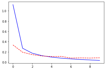
Test several MLP architectures
Define a
MultiLayerMLP([D_in, 512, 256, 128, 64, D_out])class that take the size of the layers as parameters of the constructor.Add some non-linearity with relu acivation function
class MLP(nn.Module):

    def __init__(self, d_layer):
        super(MLP, self).__init__()
        self.d_layer = d_layer
        layer_list = [nn.Linear(d_layer[l], d_layer[l+1]) for l in range(len(d_layer) - 1)]
        self.linears = nn.ModuleList(layer_list)

    def forward(self, X):
        X = X.view(-1, self.d_layer[0])
        # relu(Wl x) for all hidden layer
        for layer in self.linears[:-1]:
            X = F.relu(layer(X))
        # softmax(Wl x) for output layer
        return F.log_softmax(self.linears[-1](X), dim=1)
model = MLP([D_in, 512, 256, 128, 64, D_out]).to(device)

optimizer = optim.SGD(model.parameters(), lr=0.01, momentum=0.5)
criterion = nn.NLLLoss()

model, losses, accuracies = train_val_model(model, criterion, optimizer, dataloaders,
                       num_epochs=10, log_interval=2)

_ = plt.plot(losses['train'], '-b', losses['val'], '--r')
Epoch 0/9
----------
train Loss: 1.1216 Acc: 66.19%
val Loss: 0.3347 Acc: 90.71%

Epoch 2/9
----------
train Loss: 0.1744 Acc: 94.94%
val Loss: 0.1461 Acc: 95.52%

Epoch 4/9
----------
train Loss: 0.0979 Acc: 97.14%
val Loss: 0.1089 Acc: 96.49%

Epoch 6/9
----------
train Loss: 0.0635 Acc: 98.16%
val Loss: 0.0795 Acc: 97.68%

Epoch 8/9
----------
train Loss: 0.0422 Acc: 98.77%
val Loss: 0.0796 Acc: 97.54%

Training complete in 1m 53s
Best val Acc: 97.68%
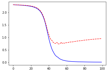
Reduce the size of training dataset
Reduce the size of the training dataset by considering only 10
minibatche for size16.
train_loader, val_loader = load_mnist(16, 1000)

train_size = 10 * 16

# Stratified sub-sampling
targets = train_loader.dataset.targets.numpy()
nclasses = len(set(targets))

indices = np.concatenate([np.random.choice(np.where(targets == lab)[0], int(train_size / nclasses),replace=False)
    for lab in set(targets)])
np.random.shuffle(indices)

train_loader = torch.utils.data.DataLoader(train_loader.dataset, batch_size=16,
    sampler=torch.utils.data.SubsetRandomSampler(indices))

# Check train subsampling
train_labels = np.concatenate([labels.numpy() for inputs, labels in train_loader])
print("Train size=", len(train_labels), " Train label count=", {lab:np.sum(train_labels == lab) for lab in set(train_labels)})
print("Batch sizes=", [inputs.size(0) for inputs, labels in train_loader])

# Put together train and val
dataloaders = dict(train=train_loader, val=val_loader)

# Info about the dataset
D_in = np.prod(dataloaders["train"].dataset.data.shape[1:])
D_out = len(dataloaders["train"].dataset.targets.unique())
print("Datasets shape", {x: dataloaders[x].dataset.data.shape for x in ['train', 'val']})
print("N input features", D_in, "N output", D_out)
Train size= 160  Train label count= {0: 16, 1: 16, 2: 16, 3: 16, 4: 16, 5: 16, 6: 16, 7: 16, 8: 16, 9: 16}
Batch sizes= [16, 16, 16, 16, 16, 16, 16, 16, 16, 16]
Datasets shape {'train': torch.Size([60000, 28, 28]), 'val': torch.Size([10000, 28, 28])}
N input features 784 N output 10
model = MLP([D_in, 512, 256, 128, 64, D_out]).to(device)
optimizer = optim.SGD(model.parameters(), lr=0.01, momentum=0.5)
criterion = nn.NLLLoss()
model, losses, accuracies = train_val_model(model, criterion, optimizer, dataloaders,
num_epochs=100, log_interval=20)
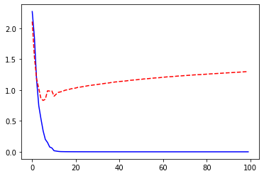
_ = plt.plot(losses['train'], '-b', losses['val'], '--r')
Epoch 0/99
----------
train Loss: 2.3050 Acc: 10.00%
val Loss: 2.3058 Acc: 8.92%

Epoch 20/99
----------
train Loss: 2.2389 Acc: 42.50%
val Loss: 2.2534 Acc: 29.90%

Epoch 40/99
----------
train Loss: 0.9381 Acc: 83.75%
val Loss: 1.1041 Acc: 68.36%

Epoch 60/99
----------
train Loss: 0.0533 Acc: 100.00%
val Loss: 0.7823 Acc: 76.69%

Epoch 80/99
----------
train Loss: 0.0138 Acc: 100.00%
val Loss: 0.8884 Acc: 76.88%

Training complete in 2m 17s
Best val Acc: 77.08%
Use an opimizer with an adaptative learning rate: Adam
model = MLP([D_in, 512, 256, 128, 64, D_out]).to(device)
optimizer = torch.optim.Adam(model.parameters(), lr=0.001)
criterion = nn.NLLLoss()

model, losses, accuracies = train_val_model(model, criterion, optimizer, dataloaders,
                       num_epochs=100, log_interval=20)

_ = plt.plot(losses['train'], '-b', losses['val'], '--r')
Epoch 0/99
----------
train Loss: 2.2706 Acc: 23.75%
val Loss: 2.1079 Acc: 44.98%

Epoch 20/99
----------
train Loss: 0.0012 Acc: 100.00%
val Loss: 1.0338 Acc: 78.23%

Epoch 40/99
----------
train Loss: 0.0003 Acc: 100.00%
val Loss: 1.1383 Acc: 78.24%

Epoch 60/99
----------
train Loss: 0.0002 Acc: 100.00%
val Loss: 1.2075 Acc: 78.17%

Epoch 80/99
----------
train Loss: 0.0001 Acc: 100.00%
val Loss: 1.2571 Acc: 78.26%

Training complete in 2m 28s
Best val Acc: 78.35%
Run MLP on CIFAR-10 dataset
The CIFAR-10 dataset consists of 60000 32x32 colour images in 10 classes, with 6000 images per class. There are 50000 training images and 10000 test images.
The dataset is divided into five training batches and one test batch, each with 10000 images. The test batch contains exactly 1000 randomly-selected images from each class. The training batches contain the remaining images in random order, but some training batches may contain more images from one class than another. Between them, the training batches contain exactly 5000 images from each class.
Load CIFAR-10 dataset
from pathlib import Path
WD = os.path.join(Path.home(), "data", "pystatml", "dl_cifar10_pytorch")
os.makedirs(WD, exist_ok=True)
os.chdir(WD)
print("Working dir is:", os.getcwd())
os.makedirs("data", exist_ok=True)
os.makedirs("models", exist_ok=True)

import numpy as np
import torch
import torch.nn as nn
import torchvision
import torchvision.transforms as transforms


# Device configuration
device = torch.device('cuda' if torch.cuda.is_available() else 'cpu')

# Hyper-parameters
num_epochs = 5
learning_rate = 0.001

# Image preprocessing modules
transform = transforms.Compose([
    transforms.Pad(4),
    transforms.RandomHorizontalFlip(),
    transforms.RandomCrop(32),
    transforms.ToTensor()])

# CIFAR-10 dataset
train_dataset = torchvision.datasets.CIFAR10(root='data/',
                                             train=True,
                                             transform=transform,
                                             download=True)

val_dataset = torchvision.datasets.CIFAR10(root='data/',
                                            train=False,
                                            transform=transforms.ToTensor())

# Data loader
train_loader = torch.utils.data.DataLoader(dataset=train_dataset,
                                           batch_size=100,
                                           shuffle=True)

val_loader = torch.utils.data.DataLoader(dataset=val_dataset,
                                          batch_size=100,
                                          shuffle=False)

# Put together train and val
dataloaders = dict(train=train_loader, val=val_loader)

# Info about the dataset
D_in = np.prod(dataloaders["train"].dataset.data.shape[1:])
D_out = len(set(dataloaders["train"].dataset.targets))
print("Datasets shape:", {x: dataloaders[x].dataset.data.shape for x in ['train', 'val']})
print("N input features:", D_in, "N output:", D_out)
Working dir is: /home/ed203246/data/pystatml/dl_cifar10_pytorch
Files already downloaded and verified
Datasets shape: {'train': (50000, 32, 32, 3), 'val': (10000, 32, 32, 3)}
N input features: 3072 N output: 10
model = MLP([D_in, 512, 256, 128, 64, D_out]).to(device)
optimizer = torch.optim.Adam(model.parameters(), lr=0.001)
criterion = nn.NLLLoss()

model, losses, accuracies = train_val_model(model, criterion, optimizer, dataloaders,
                       num_epochs=50, log_interval=10)

_ = plt.plot(losses['train'], '-b', losses['val'], '--r')
---------------------------------------------------------------------------

RuntimeError                              Traceback (most recent call last)

<ipython-input-36-13724f7cb709> in <module>
----> 1 model = MLP([D_in, 512, 256, 128, 64, D_out]).to(device)
      2 optimizer = torch.optim.Adam(model.parameters(), lr=0.001)
      3 criterion = nn.NLLLoss()
      4
      5 model, losses, accuracies = train_val_model(model, criterion, optimizer, dataloaders,


~/anaconda3/lib/python3.7/site-packages/torch/nn/modules/module.py in to(self, *args, **kwargs)
    424             return t.to(device, dtype if t.is_floating_point() else None, non_blocking)
    425
--> 426         return self._apply(convert)
    427
    428     def register_backward_hook(self, hook):


~/anaconda3/lib/python3.7/site-packages/torch/nn/modules/module.py in _apply(self, fn)
    200     def _apply(self, fn):
    201         for module in self.children():
--> 202             module._apply(fn)
    203
    204         def compute_should_use_set_data(tensor, tensor_applied):


~/anaconda3/lib/python3.7/site-packages/torch/nn/modules/module.py in _apply(self, fn)
    200     def _apply(self, fn):
    201         for module in self.children():
--> 202             module._apply(fn)
    203
    204         def compute_should_use_set_data(tensor, tensor_applied):


~/anaconda3/lib/python3.7/site-packages/torch/nn/modules/module.py in _apply(self, fn)
    222                 # `with torch.no_grad():`
    223                 with torch.no_grad():
--> 224                     param_applied = fn(param)
    225                 should_use_set_data = compute_should_use_set_data(param, param_applied)
    226                 if should_use_set_data:


~/anaconda3/lib/python3.7/site-packages/torch/nn/modules/module.py in convert(t)
    422
    423         def convert(t):
--> 424             return t.to(device, dtype if t.is_floating_point() else None, non_blocking)
    425
    426         return self._apply(convert)


RuntimeError: CUDA error: all CUDA-capable devices are busy or unavailable